Seeing sample data next to the formula and the result it produces is often the fastest way to understand VLOOKUP. This page lays out a small sample dataset, the exact formula used against it, and what gets returned, so you can compare each part directly against your own spreadsheet.
Once the example is clear, the final section shows the same match performed in Turbo Excel Lookup, for situations where the sample data below is cleaner than what you're actually working with.


| Sheet1 - Orders | ||
|---|---|---|
| Order ID | Customer ID | Customer Name (to fill) |
| 1001 | C-204 | ? |
| 1002 | C-118 | ? |
| Sheet2 - Customers | |
|---|---|
| Customer ID | Customer Name |
| C-118 | Priya Nair |
| C-204 | Daniel Osei |
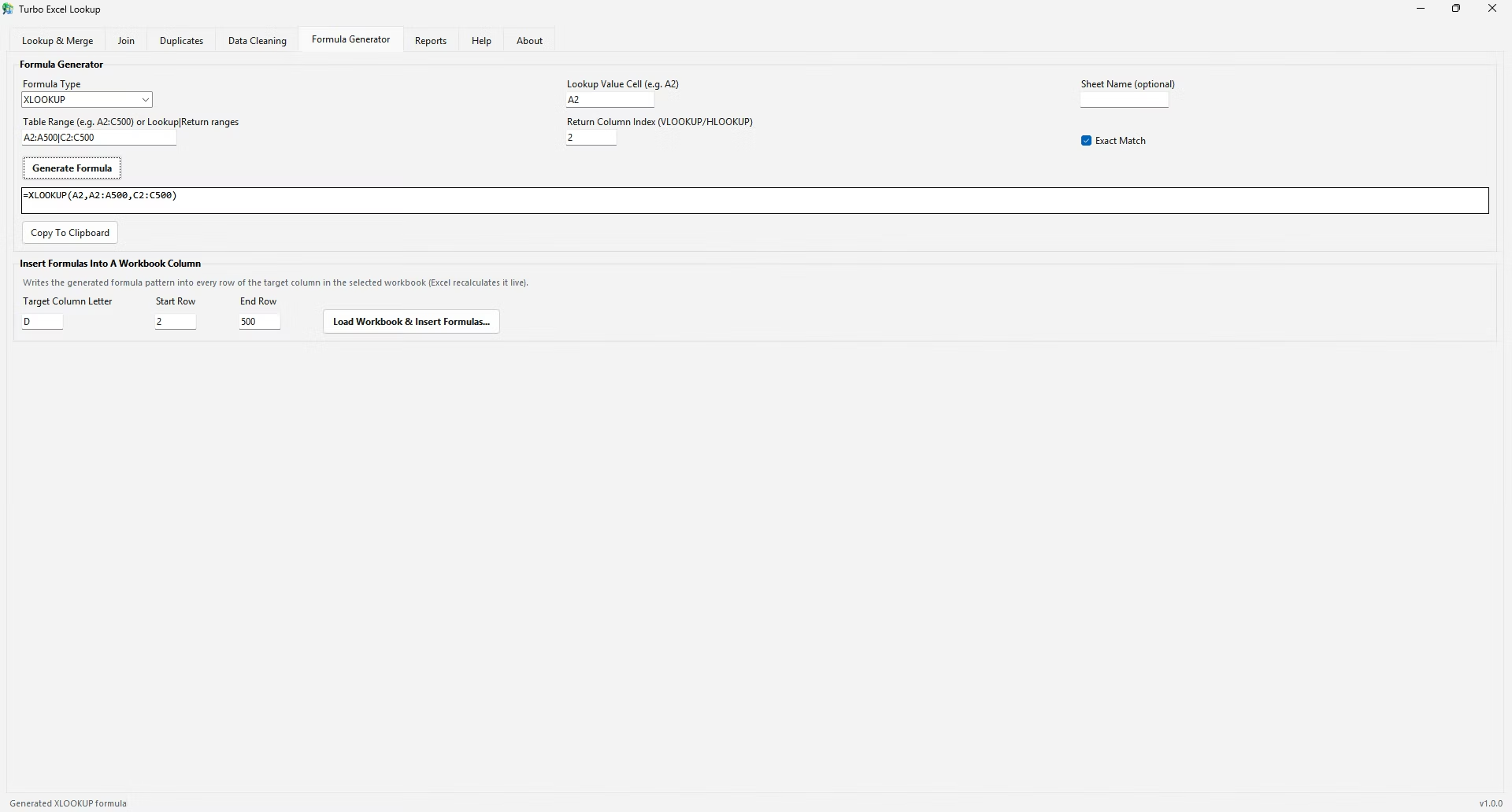
Placed in C2 of Sheet1, this formula takes the Customer ID in B2 ("C-204"), searches for it in column A of the Customers sheet, and returns the matching value from column B. The result in C2 is "Daniel Osei". Notice the Customers sheet isn't sorted by Customer ID, which is fine here because FALSE forces an exact match rather than relying on sort order.
Copying this formula into C3 with a locked range (Sheet2!$A:$B) correctly returns "Priya Nair" for Customer ID C-118, demonstrating that the row order in the lookup table doesn't matter for exact-match VLOOKUP.
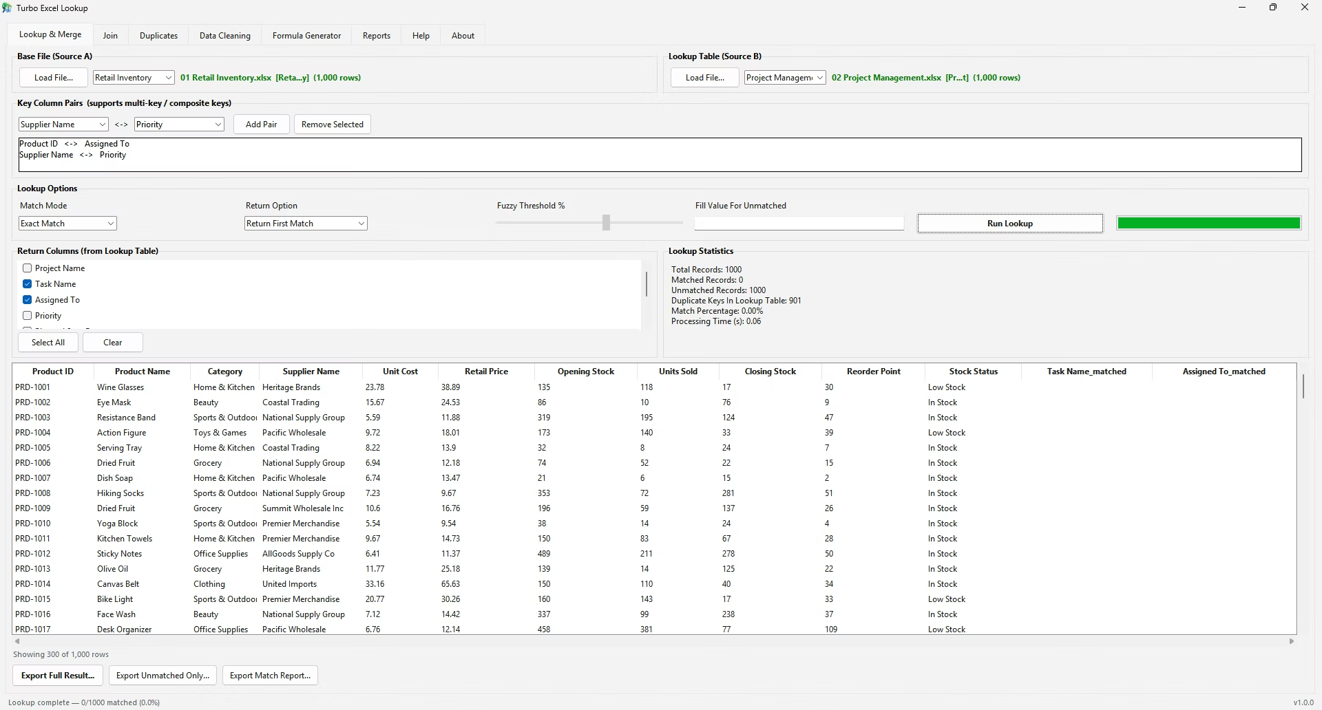
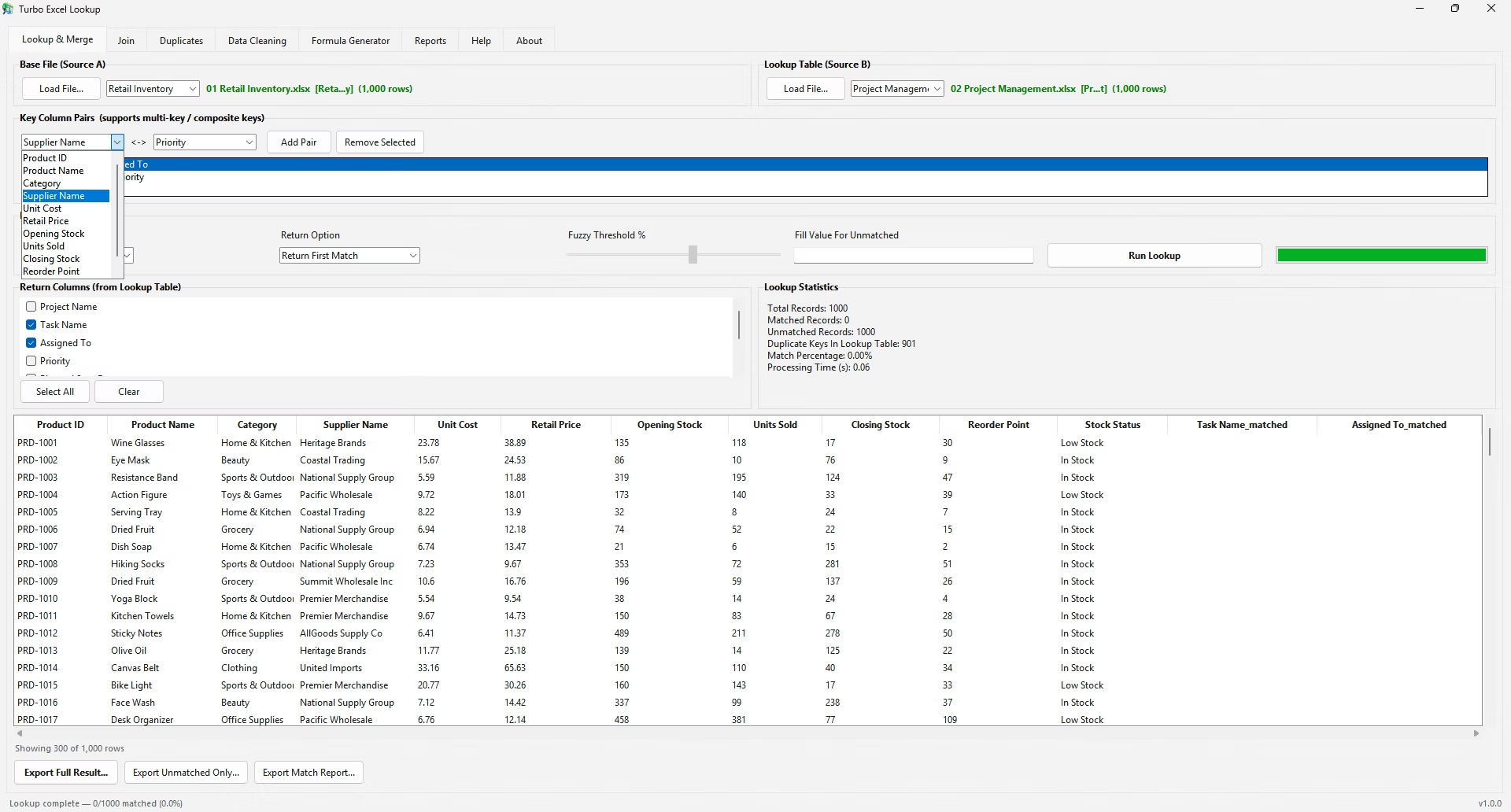
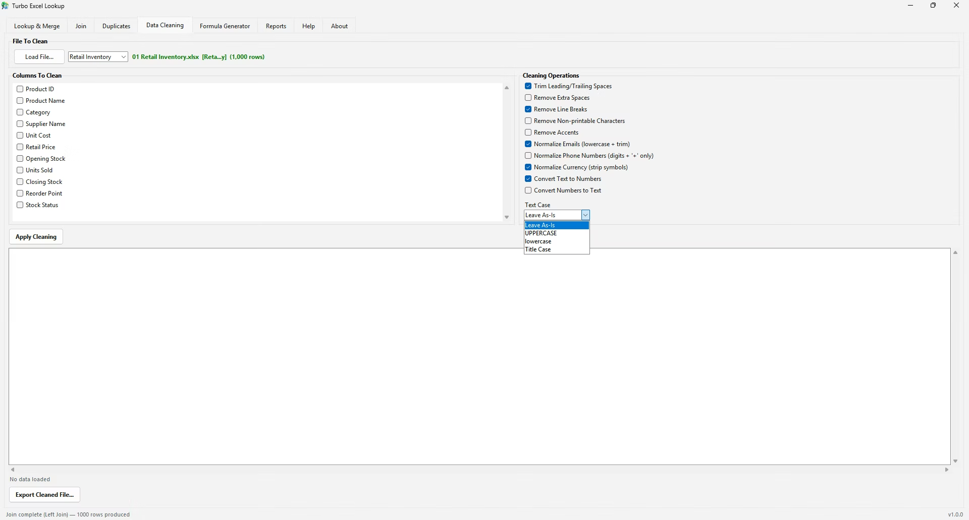
In Turbo Excel Lookup, this exact scenario is a two-file, single-key lookup: Orders as the Base File, Customers as the Lookup Table, Customer ID matched to Customer ID, with Customer Name ticked as the column to return. The app produces the same C-204 → Daniel Osei and C-118 → Priya Nair results, but also shows a match-rate statistic - useful once your real order sheet has thousands of rows instead of two, some of which may not have a corresponding customer record.
Building on the Orders and Customers example, suppose a third order arrives with Customer ID "C-350", which doesn't exist anywhere in the Customers sheet. Copying the same locked formula into that row returns #N/A rather than a name, correctly signaling that this customer record is missing rather than silently leaving the cell blank or guessing at a value.
This is a useful property of exact-match VLOOKUP - it fails loudly rather than quietly, which is generally the safer behavior for financial or customer-facing data. In Turbo Excel Lookup, the same missing customer would show up in the Unmatched export and be reflected in the match-percentage statistic, making it just as visible but without needing to scroll through the sheet hunting for #N/A manually.
If a formula built the same way as this example still returns unexpected errors on your own data, the most likely causes are hidden characters copied in from another system, a lookup column that isn't actually the leftmost column selected, or a data type mismatch between what looks like the same value in both sheets. Checking these three specific possibilities, in that order, resolves the majority of cases that don't match the clean behavior shown in the example above.
The Customer ID and Customer Name column names used in this example are placeholders - when adapting the same structure to your own data, only the column letters and the col_index_num need to change, while the overall formula shape (lookup_value, locked table_array, column number, FALSE) stays identical regardless of what the columns are actually named. Recognizing this - that the formula's structure is independent of the specific field names involved - makes it much faster to adapt a worked example to a new, unrelated dataset.
A worked example with concrete sample data, checked against the formula's actual output, is the clearest way to confirm a VLOOKUP formula is behaving correctly before applying it to real, larger data. Keep this pattern in mind as a quick sanity check for any new lookup formula you build.
Does the lookup table need to be sorted for this example to work?
No, because the formula uses FALSE for an exact match. Sorting only matters when using TRUE for an approximate match.
What if Customer ID C-204 appeared twice in the Customers sheet?
VLOOKUP would return only the first occurrence it encounters. If both records might legitimately need to be seen, Turbo Excel Lookup's Return All Matches option would concatenate them together instead.
Can I use this same formula pattern with text-based IDs?
Yes, VLOOKUP works the same way whether the lookup value is a number or text, as long as the data types match between the lookup value and the table.
How would I adapt this example to two separate files rather than two sheets?
The formula syntax is nearly identical but references an external workbook, e.g. '[Customers.xlsx]Sheet1'!A:B, and both files generally need to be open for the formula to calculate reliably.
What should I do when a VLOOKUP result is #N/A because the record genuinely doesn't exist?
That's expected, correct behavior - it's telling you the lookup value has no match in the table, which may mean the record needs to be added to the source table or investigated separately.
Is there a faster way to see all unmatched rows at once?
Filtering the result column for #N/A/errors works in Excel; Turbo Excel Lookup can export just the unmatched rows directly as their own file after a lookup runs.
What are the three most likely causes if my own VLOOKUP doesn't match this example's behavior?
Hidden characters from copied or imported data, a lookup column that isn't actually the leftmost column in the selected range, and a data type mismatch such as text versus number.
Do I need to change the whole formula structure to match my own column names?
No, only the range references and column index number need to change - the overall formula shape stays the same regardless of what your columns are actually named.
Ready to stop fighting #N/A errors and match your spreadsheets visually?