Excel VLOOKUP Formula

The VLOOKUP formula is one of the most widely used functions in Excel, built specifically to search for a value in the leftmost column of a range and return a related value from another column in the same row. It has been the go-to solution for pulling a price from a price list, a name from an employee roster, or a status from a tracking sheet for more than two decades, and it remains the first function most people learn once they move past basic arithmetic in a spreadsheet.

Despite its popularity, the VLOOKUP formula has a reputation for being finicky. A single extra space, a mismatched data type, or a column that gets inserted in the wrong place is enough to turn a working formula into a wall of #N/A errors. This page breaks down exactly how the formula works, argument by argument, and also introduces Turbo Excel Lookup, a Windows desktop app that performs the same lookup logic visually, without requiring you to write or debug a single formula.

Every VLOOKUP formula takes four arguments, and understanding each one is the key to avoiding errors:

• lookup_value - the value you're searching for, usually a cell reference like A2.
• table_array - the full range of cells that contains both the lookup column and the column you want returned. The lookup value must sit in the first column of this range.
• col_index_num - the column number within table_array to pull the result from, counted from left to right starting at 1.
• [range_lookup] - optional. Use FALSE (or 0) for an exact match, which is what most spreadsheet work needs, or TRUE for an approximate match against a sorted list.

A typical formula looks like =VLOOKUP(A2, Sheet2!A:D, 3, FALSE), which searches for the value in A2 within column A of Sheet2, and returns the corresponding value from the third column of that range.

VLOOKUP only searches the leftmost column of the range you give it, which means the moment your data is laid out differently, you're stuck rearranging columns or nesting it inside other functions. It also fails silently on anything less than an exact character match - trailing spaces, inconsistent capitalization, or accented characters all produce #N/A even though a human would immediately recognize the values as the same.

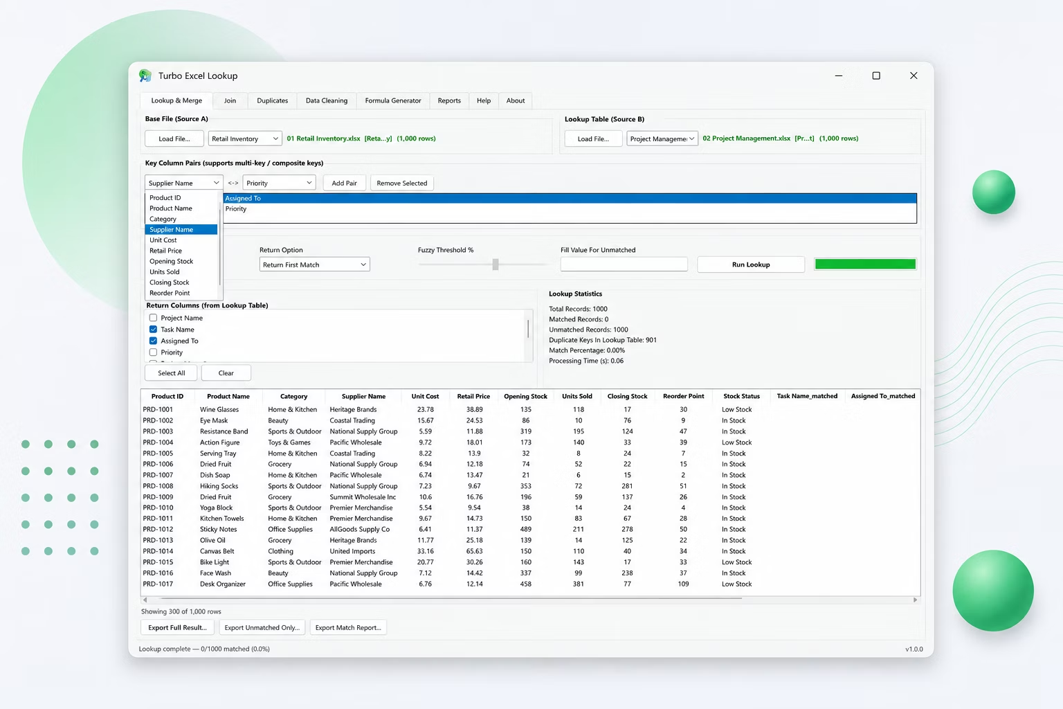
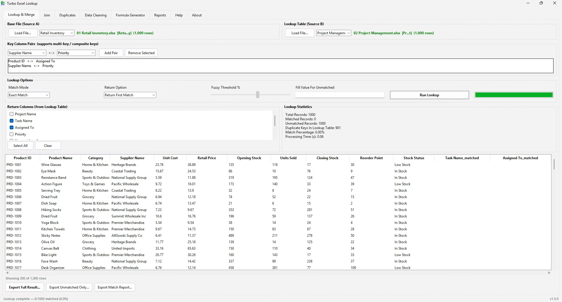
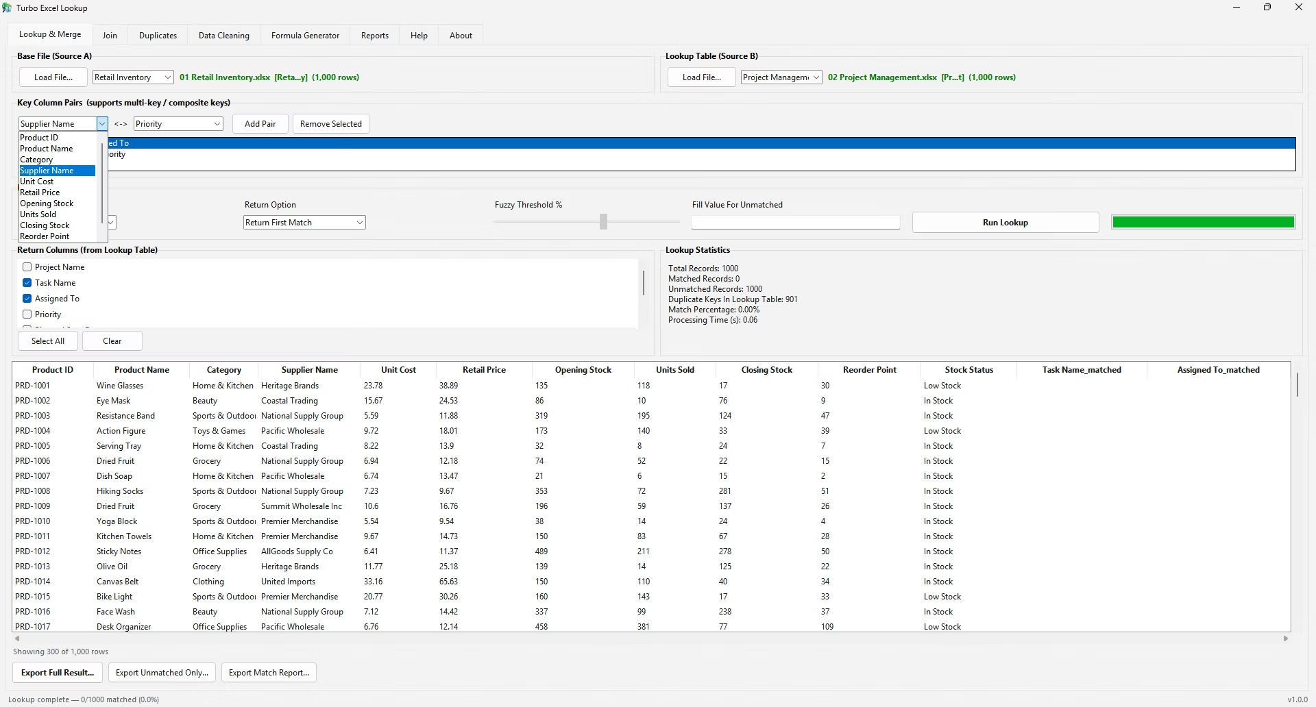
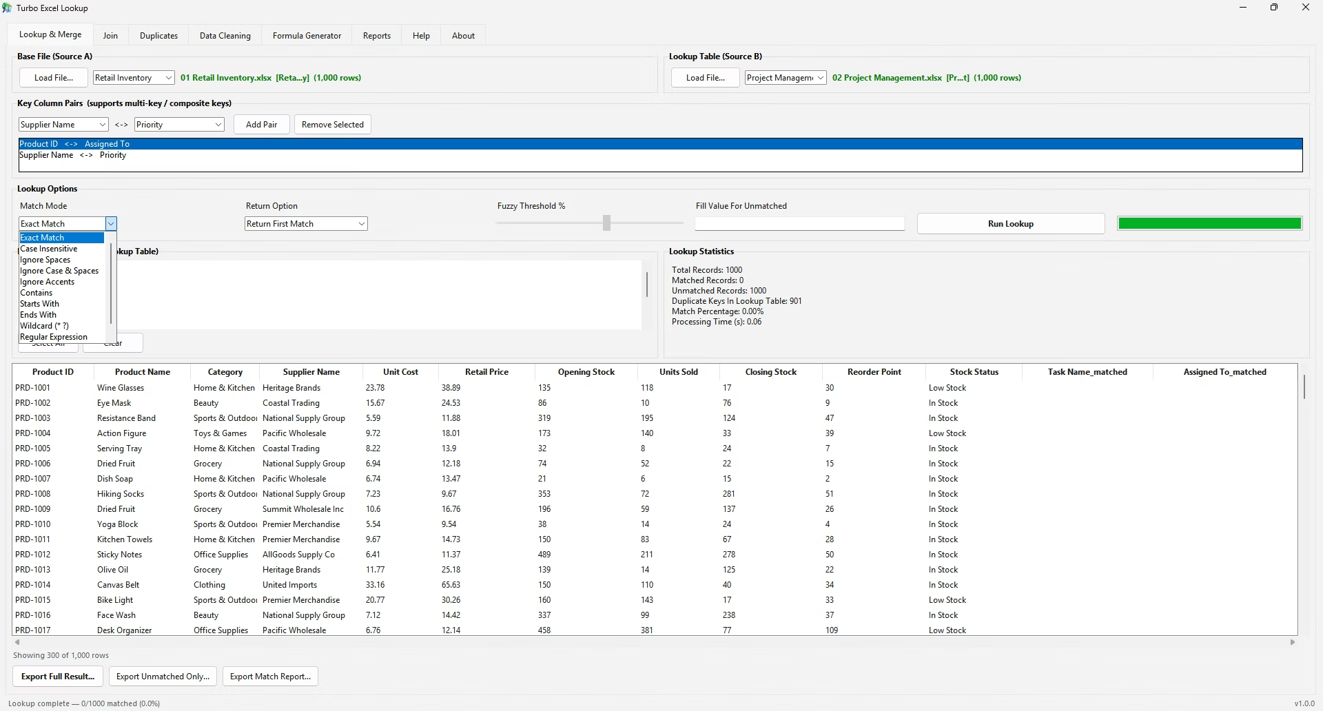
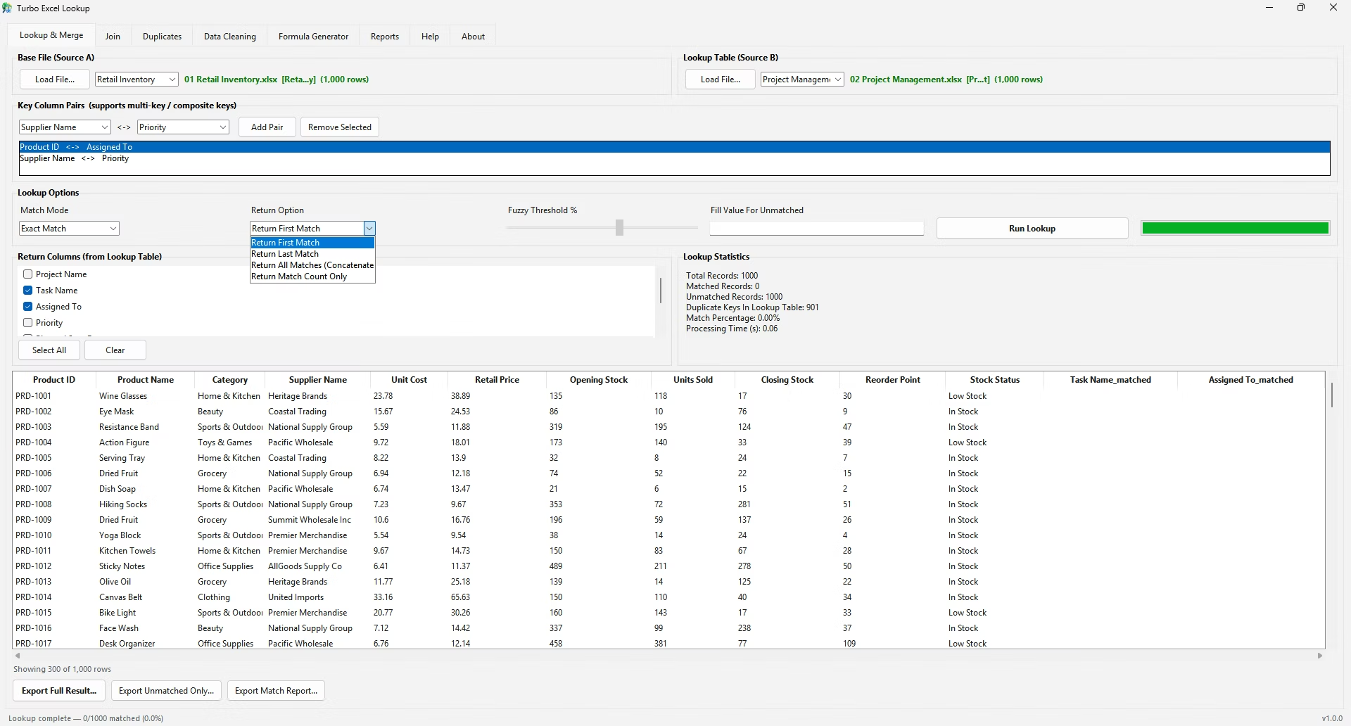
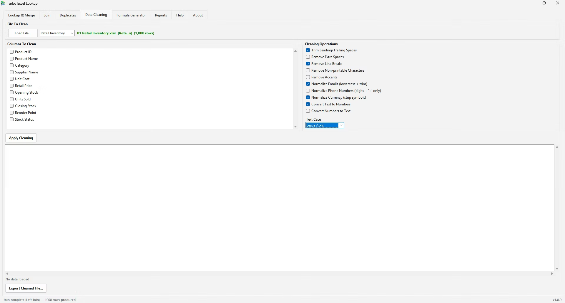
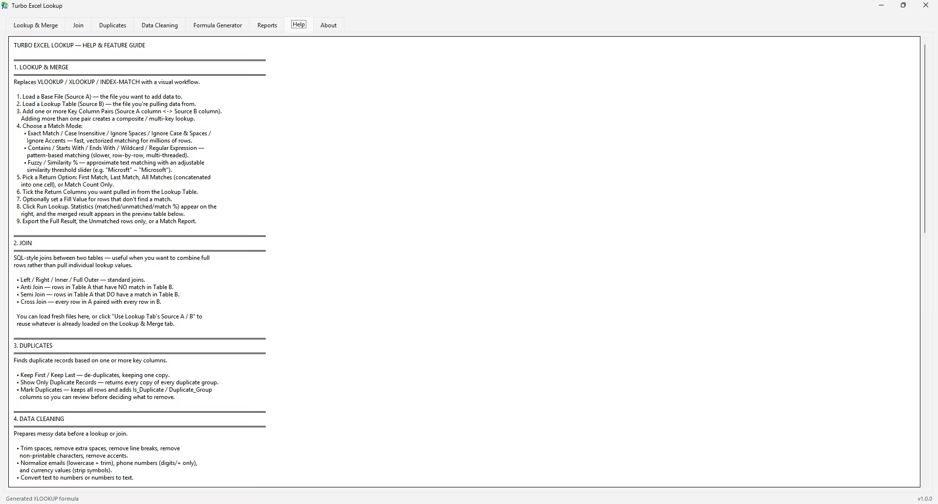
Turbo Excel Lookup was built around exactly this pain point. Its Lookup & Merge tab reproduces the VLOOKUP mental model - pick a base file, pick a lookup table, choose the matching columns - but adds eleven match modes, including Case Insensitive, Ignore Spaces, and Ignore Accents, so the kind of messy real-world text that breaks a formula still matches correctly. There's no column-order requirement either; you simply tick whichever columns you want pulled back.

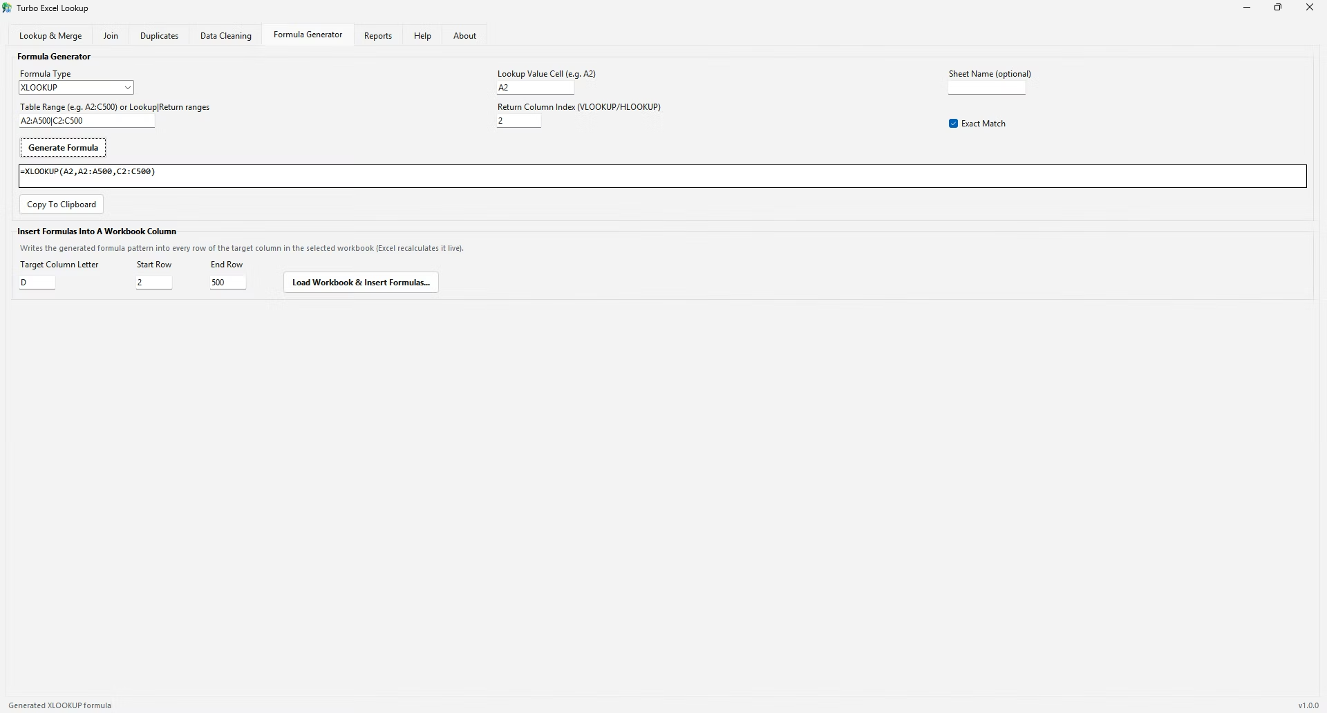
A live, recalculating formula is still the right call when a workbook needs to update automatically as new rows are typed into it by someone else. For that case, Turbo Excel Lookup's Formula Generator tab builds the exact VLOOKUP syntax for you from the lookup cell, the table range, and the column index, and can write it directly into every row of a target column so the workbook keeps recalculating natively in Excel.

This gives you both approaches in one app: run a one-off, high-accuracy match through the visual workflow when you just need the data joined, or generate a proper formula string when the file needs to stay live.

The TRUE setting for range_lookup is worth understanding even though FALSE is the safer default for most work. In approximate match mode, VLOOKUP doesn't require an identical value - it finds the largest value in the lookup column that is less than or equal to your lookup_value, provided that column is sorted in ascending order. This is genuinely useful for bucketed data, such as converting a numeric score into a letter grade or a shipping weight into a price tier, where you're matching a range rather than a single point value.

The risk is that if the lookup column isn't actually sorted, approximate match doesn't throw an error - it simply returns whatever value happens to fall in the wrong place, which can go unnoticed for a long time in a shared workbook. Because Turbo Excel Lookup's Match Modes are explicit choices rather than a TRUE/FALSE toggle, this particular failure mode - forgetting to sort data that approximate match silently depends on - doesn't arise in the same way.

VLOOKUP sits alongside a small family of related lookup functions that solve overlapping problems in slightly different ways. INDEX/MATCH removes the leftmost-column restriction that VLOOKUP has, at the cost of combining two functions instead of one. XLOOKUP, covered in detail elsewhere on this site, modernizes the whole concept further but requires a recent Excel version. HLOOKUP mirrors VLOOKUP exactly but searches rows instead of columns. Knowing this family exists helps when VLOOKUP's specific limitations - column order, single-column returns, Excel version - genuinely don't fit a particular sheet's layout.

In a shared workbook maintained by more than one person, VLOOKUP formulas tend to drift out of consistency over time - one person locks their ranges, another doesn't; one person always uses FALSE, another occasionally forgets. Establishing a short, written convention for how lookups should be built in a given workbook, even something as simple as a one-line note in a README tab, keeps the formulas predictable for everyone who touches the file. This kind of convention becomes less necessary with Turbo Excel Lookup, since its Match Modes and Fill Value settings are chosen consistently through the same interface every time, rather than depending on each person remembering the same formula habits independently.

VLOOKUP remains one of the most dependable tools in Excel once its four arguments and its leftmost-column requirement are understood clearly. For clean, well-structured data it's often still the fastest option available. The moment your own data stops being clean, though, is exactly when a dedicated matching tool like Turbo Excel Lookup starts paying for itself in saved troubleshooting time.