Reading a VLOOKUP formula's syntax in the abstract rarely makes it click - seeing each argument mapped onto a real table usually does. This page uses a small employee table as a running example, matching each part of the formula to the actual cells it refers to.
Once the mapping between formula and data is clear, writing new VLOOKUP formulas from scratch for different tables becomes much more straightforward.

Here's the data used throughout this page, listed in a standard range starting at cell A1:
| Employee ID | Name | Department | Salary |
|---|---|---|---|
| E101 | Asha Rao | Marketing | 54000 |
| E102 | Vikram Shah | Finance | 61000 |
| E103 | Priya Nair | Sales | 48000 |
The task is to find the Salary for employee E103. lookup_value is "E103" - the value we're searching for in column A. table_array is A2:D4 - the range containing all the data, starting from the Employee ID column.
col_index_num is 4 because Salary is the fourth column in that range, and FALSE requires an exact ID match rather than an approximate one.
To return Department instead of Salary for the same employee, only col_index_num changes, since Department is the third column in the same range:
Notice that lookup_value, table_array, and range_lookup all stay exactly the same - only the column count changes.
In practice, the lookup_value is usually a cell reference rather than typed text, so the formula updates automatically as the reference cell changes:
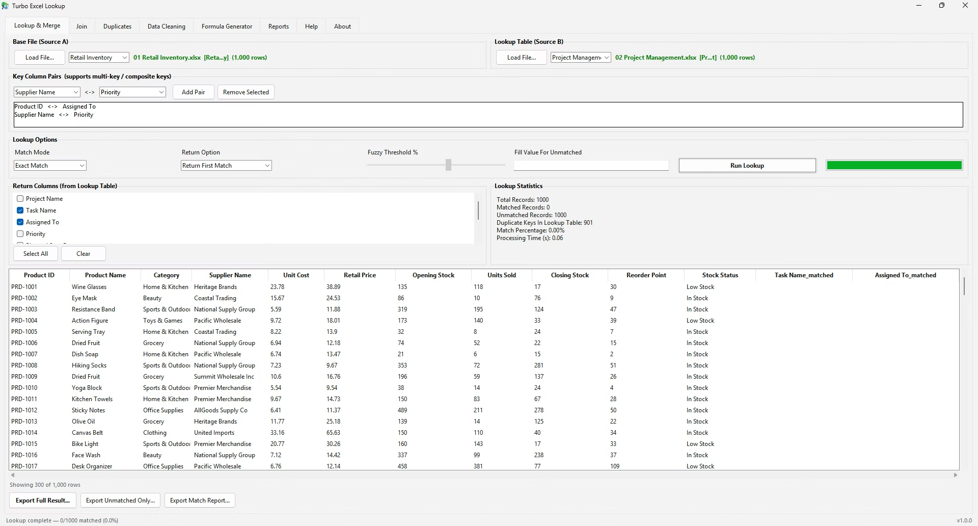
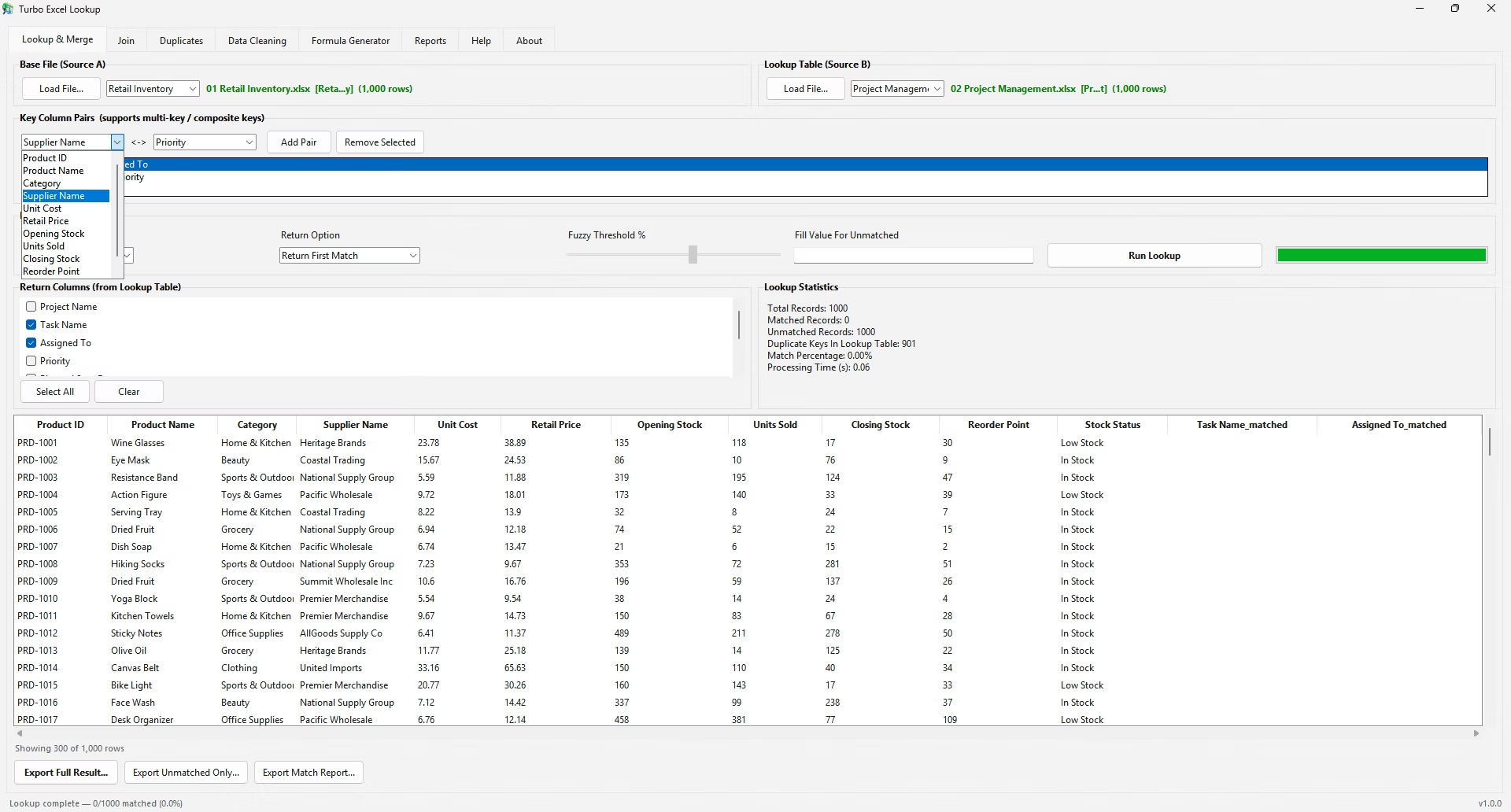
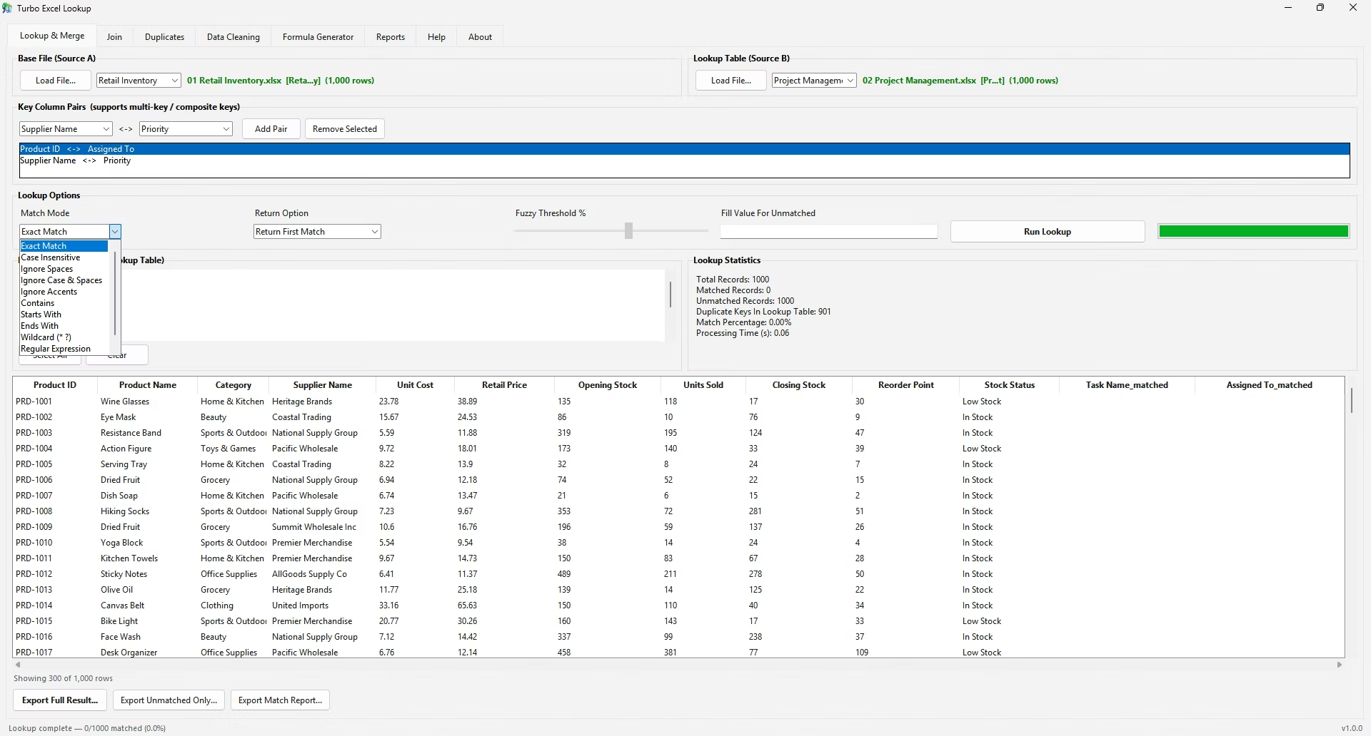
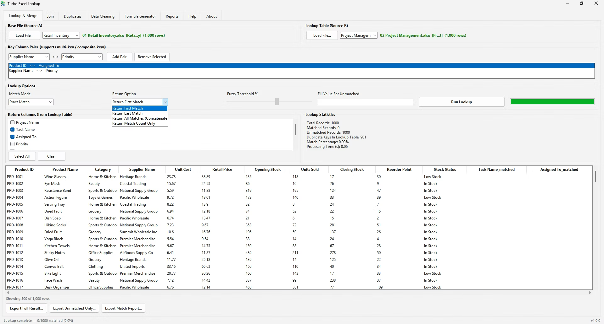
This same matching pattern - find an ID, return a column from the matching row - is exactly what Turbo Excel VLookup automates across two entire files, without needing the formula rewritten for each column you want to bring across.
A worksheet with thousands of VLOOKUP formulas recalculating against a large table_array can slow Excel down noticeably, especially if the range isn't locked and Excel has to re-evaluate a shifting reference on every keystroke.
Converting the source range into an Excel Table (Insert > Table) before referencing it in VLOOKUP tends to help, since Table references automatically resize with the data and stay consistent without needing manual $ locking.
Before applying a new VLOOKUP formula to an entire column, it's worth testing it on a single row and manually verifying the result against the source data, since a mistake caught in one cell takes seconds to fix, while the same mistake copied down five hundred rows takes much longer to untangle.
This is especially worth doing whenever the source table_array has changed shape recently, since a resized or reordered table is the single most common reason a previously reliable formula starts returning unexpected results.
What does the table_array need to include?
Every column from the lookup column through the furthest column you might want to return, since col_index_num counts from its start.
How does col_index_num change if I want a different column returned?
It changes to match the position of the new column within the same table_array - nothing else in the formula needs to change.
Should lookup_value be typed as text or referenced from a cell?
A cell reference is generally more practical, since it lets the formula update automatically as the reference cell changes.
Why does the example use FALSE and not TRUE?
Because IDs need an exact match; TRUE would allow an approximate match, which isn't appropriate for unique identifiers.
Can the same table_array be reused for multiple VLOOKUP formulas?
Yes, the same table_array can be reused across several formulas that each return a different column.
Is there a way to return several columns from a single match?
Turbo Excel VLookup lets you tick multiple columns to return in a single matching action instead of writing one formula per column.
Should I test a new formula on one row before applying it everywhere?
Yes, verifying a single result against the source data first catches setup mistakes before they're copied across an entire column.
Is it a good idea to edit source data while formulas are actively referencing it?
It's safer to keep a stable source sheet separate from a working sheet, since editing referenced data mid-use can produce confusing intermediate results.
Why would a text-formatted number fail to match a real number?
Excel treats text and numeric values as different data types, so "101" stored as text won't match 101 stored as a number even though they display the same.
Does locking a range with F4 change how the formula calculates?
No, it only fixes the range so it doesn't shift when the formula is copied - the calculation itself works the same either way.
Ready to stop fighting #N/A errors and match your spreadsheets visually?