A basic XLOOKUP matches on a single value, but many real lookups need to match on two or more conditions at once - for example, finding a price that depends on both a product and a region. XLOOKUP handles this by combining an array expression directly inside lookup_array.
This page covers that technique using an order table where both Customer Name and City together identify the correct row.






In this order table, Customer Name alone isn't guaranteed to be unique across a larger dataset, so matching also needs to check City:
| Order ID | Customer Name | City | Status |
|---|---|---|---|
| ORD-501 | Rohan Gupta | Chennai | Shipped |
| ORD-502 | Meera Pillai | Bengaluru | Pending |
| ORD-503 | Arjun Nair | Hyderabad | Delivered |
Instead of referencing a single column, lookup_array is built as an array expression that concatenates two columns together, matched against a similarly concatenated lookup value:
B2:B4&C2:C4 creates a temporary array where each row combines its Customer Name and City into one string, such as "Rohan GuptaChennai". As long as the search value F2&F3 is built the same way, XLOOKUP can match the combined string exactly, effectively matching on both columns at once.
Concatenating without a separator can occasionally create accidental matches between different value combinations. Adding a separator character reduces that risk:
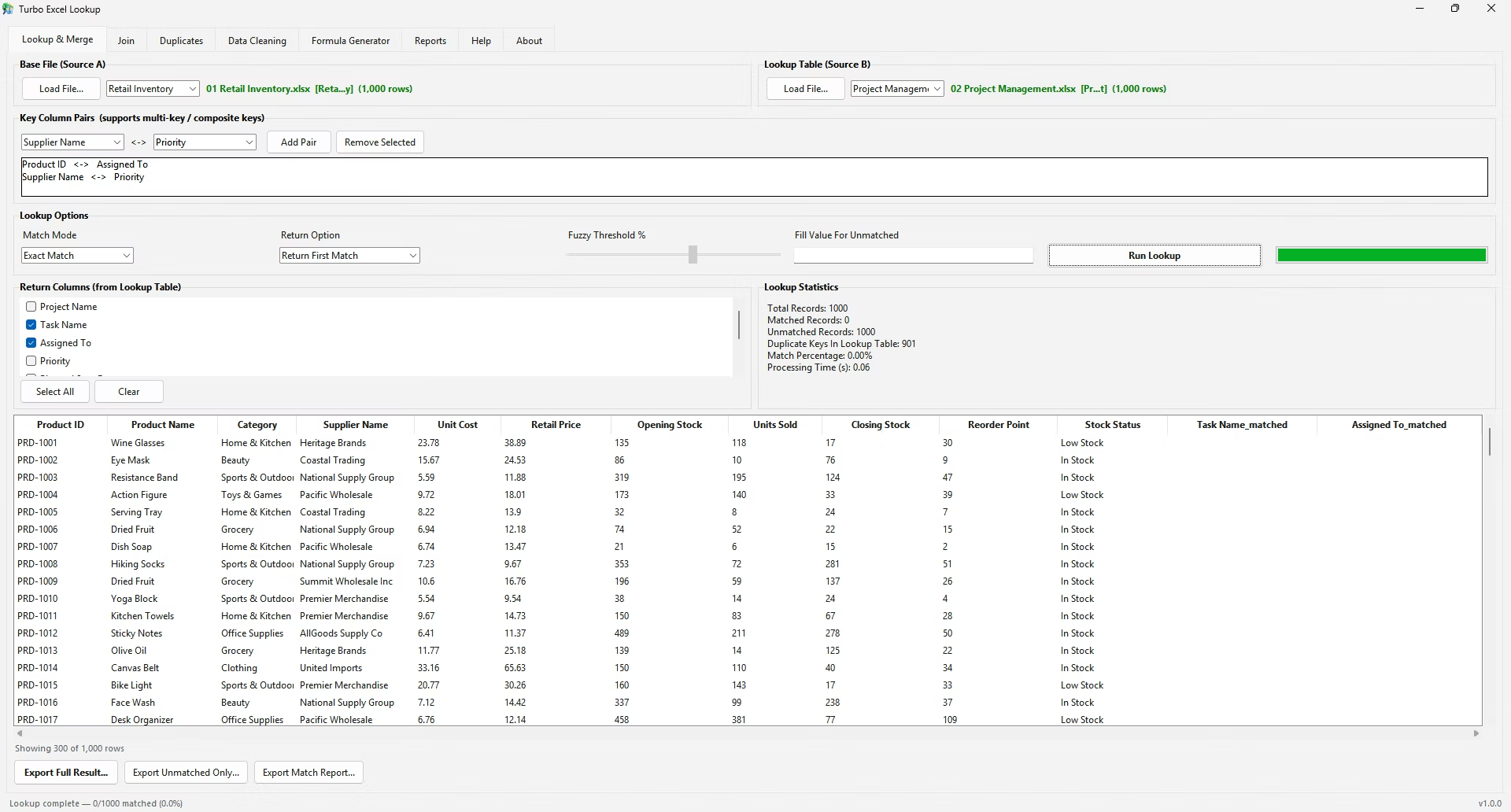
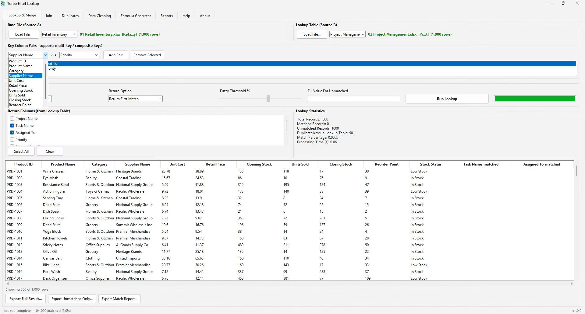
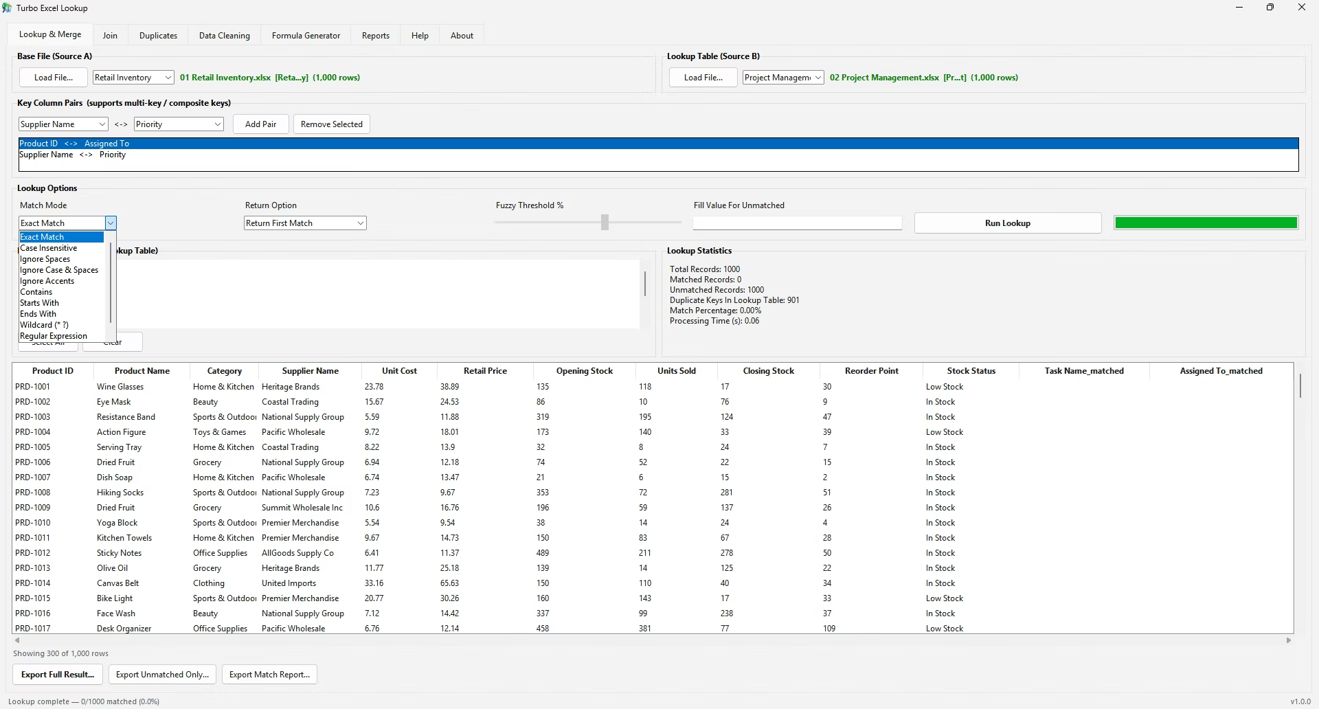
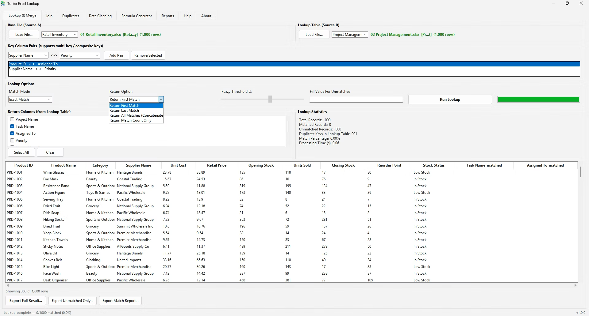
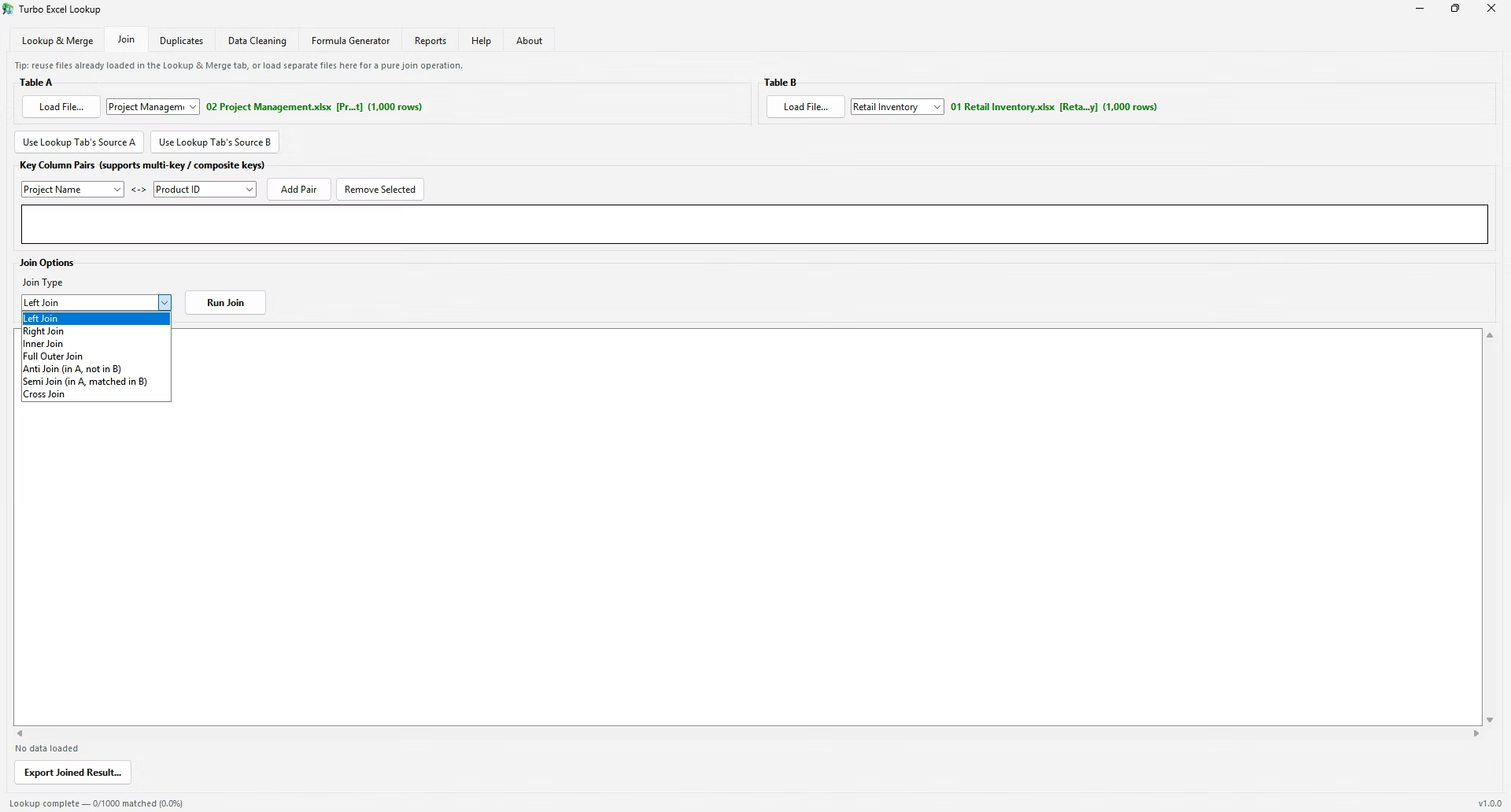
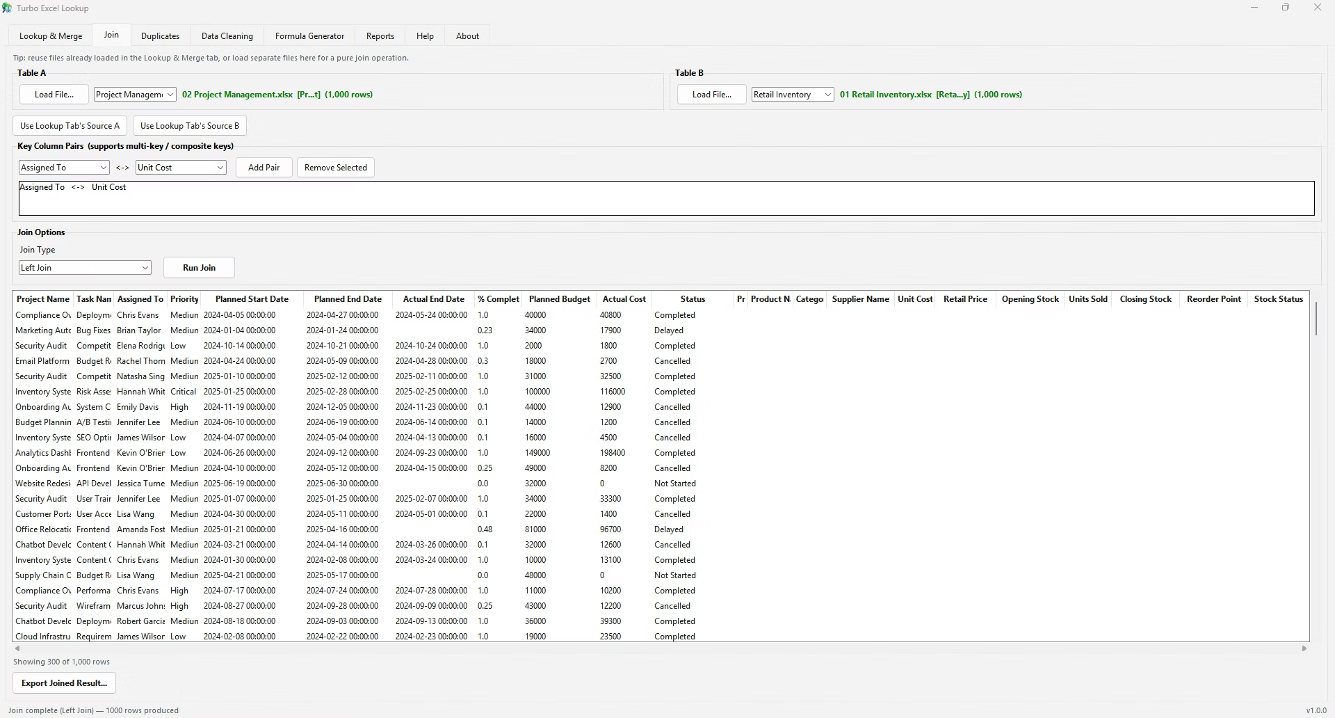
Turbo Excel VLookup supports matching on multiple key columns directly through its Key Column Pairs feature, building a composite match from several columns without needing an array formula or a manually built separator string.
Just like VLOOKUP, XLOOKUP will fail to match values that look identical but are stored as different data types - text versus number is the most common culprit.
If a lookup that should clearly match is instead falling through to if_not_found, converting the lookup value with VALUE() or TEXT() to match the source column's format usually resolves it.
A short comment or adjacent label explaining what an XLOOKUP formula is matching and why makes a shared workbook far easier to maintain, especially once several lookups start feeding into each other across different sheets.
XLOOKUP's optional fifth argument, match_mode, defaults to an exact match, but it also supports approximate matches - either the next smaller or next larger value when no exact match exists - by passing -1 or 1 instead of the default 0.
This is useful for scenarios like matching a score against grade thresholds, where an exact match won't always exist but the closest applicable bracket still needs to be found.
Can XLOOKUP match on more than one condition by default?
Not directly - it requires combining multiple columns into a single array expression inside lookup_array.
How does the ampersand (&) help with multiple criteria?
It concatenates values from multiple columns into one combined string that can then be matched as a single value.
Why add a separator character between concatenated values?
To prevent accidental matches where different value combinations happen to produce the same combined string.
Does this approach need to be entered as an array formula?
In current Excel with dynamic arrays it enters normally; in older versions it may require Ctrl+Shift+Enter.
Is there a simpler way to match on multiple columns?
Yes, Turbo Excel VLookup supports matching on several key columns directly without needing a concatenated array formula.
Does this multi-criteria approach work the same way with VLOOKUP?
A similar concatenation trick works with VLOOKUP, though XLOOKUP's independent ranges make it somewhat more straightforward to set up.
Is it a good idea to edit source data while formulas are actively referencing it?
It's safer to keep a stable source sheet separate from a working sheet, since editing referenced data mid-use can produce confusing intermediate results.
Why would a text-formatted number fail to match a real number?
Excel treats text and numeric values as different data types, so "101" stored as text won't match 101 stored as a number even though they display the same.
Does locking a range with F4 change how the formula calculates?
No, it only fixes the range so it doesn't shift when the formula is copied - the calculation itself works the same either way.
What's a fast way to check what a formula is actually returning?
Selecting part of the formula in the formula bar and pressing F9 shows its calculated value directly, without changing the formula.
Ready to stop fighting #N/A errors and match your spreadsheets visually?