XLOOKUP With Multiple Criteria

Matching on multiple criteria means the lookup needs more than one field to agree before a row is considered a match - for example, both a Product Code and a Warehouse Location need to line up, not just one or the other. XLOOKUP handles this through boolean array multiplication rather than the text-concatenation approach some guides recommend, and understanding both methods helps you pick the more reliable one for your data.

This page covers the boolean-array technique in detail, then shows Turbo Excel Lookup's native multi-key matching as a more direct alternative.

This formula compares column A to A2 and column B to B2 across every row, producing an array of TRUE/FALSE values for each condition. Multiplying the two arrays together converts TRUE/FALSE into 1/0, so a row only produces a 1 when both conditions are true simultaneously. XLOOKUP then searches this array for the value 1, and returns the corresponding row from column C.

Unlike joining two fields into a single text string with &, the boolean array method compares each field independently, avoiding the date-format and data-type mismatches that concatenation can introduce. It also scales more predictably to a third or fourth criterion - simply multiply in another comparison array, e.g. (Data!A:A=A2)*(Data!B:B=B2)*(Data!D:D=D2) - without needing to reformat anything for a combined text comparison.

The trade-off is that this formula is harder to read at a glance and can be slower on very large ranges, since Excel evaluates three or more full-column array comparisons on every recalculation.

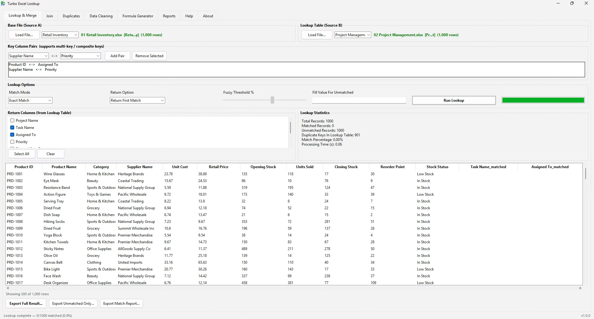
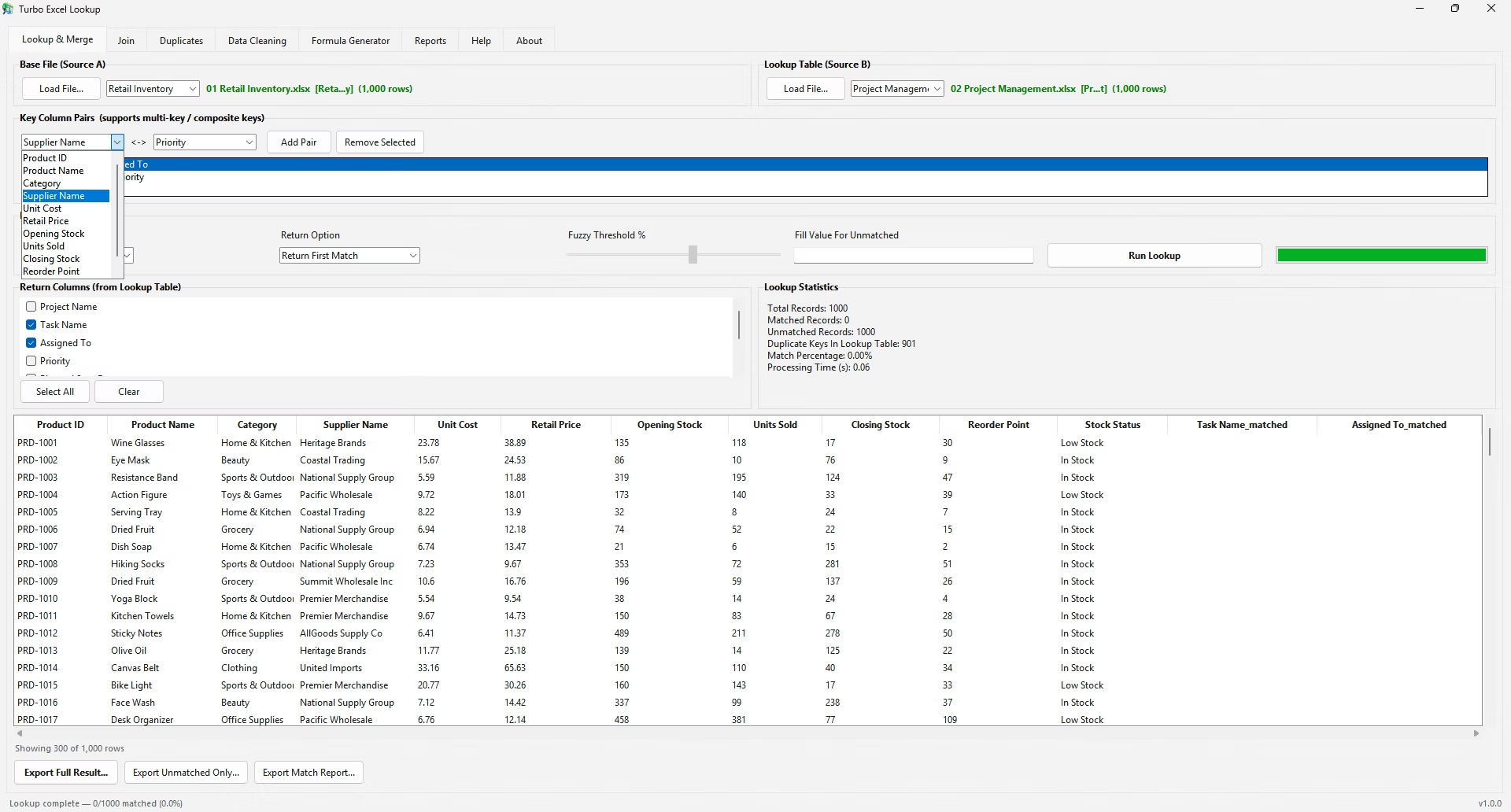
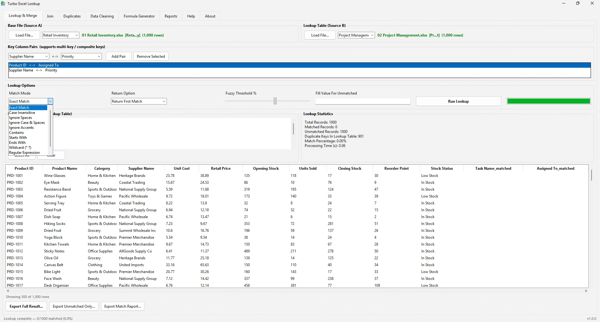
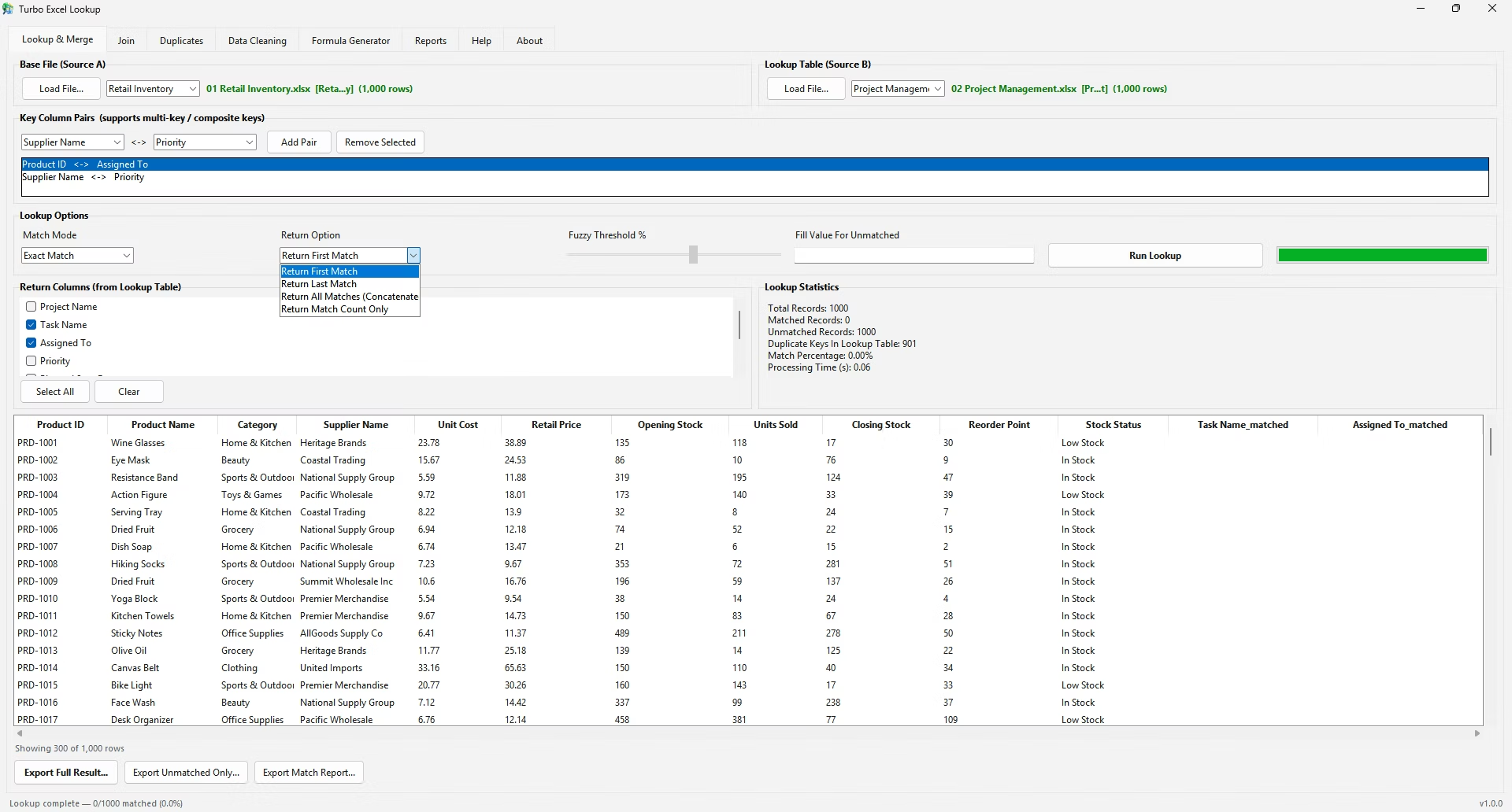
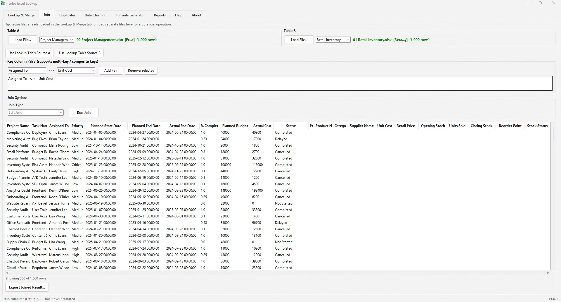
Turbo Excel Lookup's Key Column Pairs achieve the same boolean-AND matching logic - every pair added must agree for a row to count as a match - without requiring any array formula construction. Each pair is also independently assigned its own Match Mode, so one field can require an exact match while another tolerates case differences, something that isn't practical to express within a single boolean-array formula.

Because multi-criteria formulas are harder to read at a glance, it's worth deliberately testing them against a row where you know both criteria should match, and a second row where only one of the two criteria matches, to confirm the formula correctly rejects the partial match. A formula that appears to work on the first test row can still have a logic error that only becomes apparent when one condition is true and the other is false.

Turbo Excel Lookup's match-percentage report after running a multi-key lookup provides a similar sanity check at the dataset level - if the percentage is much lower than expected, it's a signal to review whether all the intended Key Column Pairs and their Match Modes are configured correctly before trusting the result.

Boolean array formulas like the one described above evaluate every row in the referenced ranges on every recalculation, which can add up in a workbook with many such formulas across a large dataset. Bounding the ranges to the actual data extent, rather than referencing whole columns, and minimizing how many multi-criteria formulas run simultaneously in one workbook both help keep recalculation times reasonable as the sheet grows.

For some multi-criteria matching needs - particularly ones involving aggregation, like summing values that meet two conditions rather than pulling a single related record - a Pivot Table or SUMIFS formula is a better fit than XLOOKUP, which is designed to return a single matching row's data rather than aggregate across several matching rows. Recognizing whether the task is really a lookup (find one related record) or an aggregation (summarize several matching records) determines which tool is the right one from the start.

The boolean array technique is the most reliable formula-based way to match on multiple criteria with XLOOKUP, avoiding the format mismatches that plain concatenation can introduce. It's still meaningfully more complex than a single-criterion lookup, which is worth factoring in when deciding how to approach a given task.