Some VLOOKUP examples try to demonstrate every possible feature at once, which can make the core idea harder to follow rather than easier. This page uses a deliberately small, simple product list with just three rows, so each of the four arguments can be traced without distraction.
Once this simple version makes sense, applying the same pattern to a larger, real spreadsheet is mostly a matter of adjusting the range.
Three products, four columns - nothing more:
| SKU | Product Name | Category | Price |
|---|---|---|---|
| SKU-2201 | Wireless Mouse | Electronics | 699 |
| SKU-2202 | Desk Lamp | Home | 899 |
| SKU-2203 | Notebook Pack | Stationery | 150 |
To find the Price of SKU-2201:
That's the whole formula. "SKU-2201" is what to search for, A2:D4 is where to search, 4 is which column to bring back, and FALSE means it has to match exactly.
A good way to build confidence is to change one argument at a time and observe the result. Changing the lookup_value to "SKU-2203" returns 150 instead of 699. Changing col_index_num from 4 to 3 returns the Category instead of the Price for the same product.
There's no sorting requirement, no approximate matching, and no multi-sheet references involved - just a flat table and an exact-match lookup. That's intentional, since those additions are worth learning only after the basic four-argument pattern is second nature.
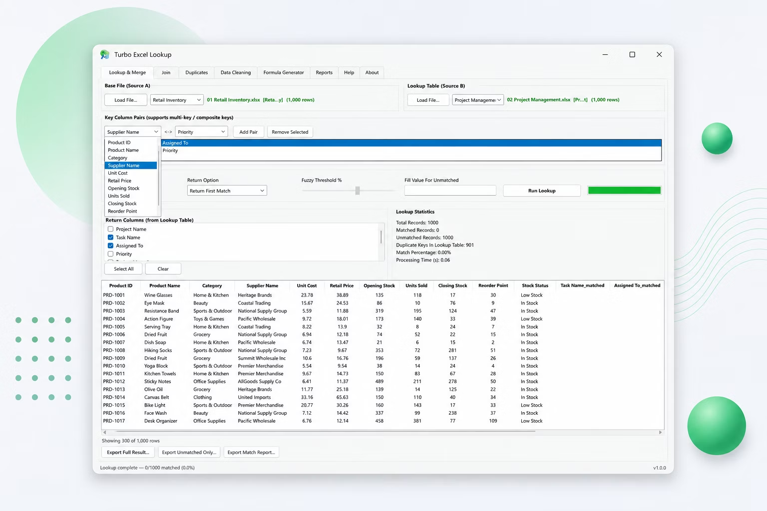
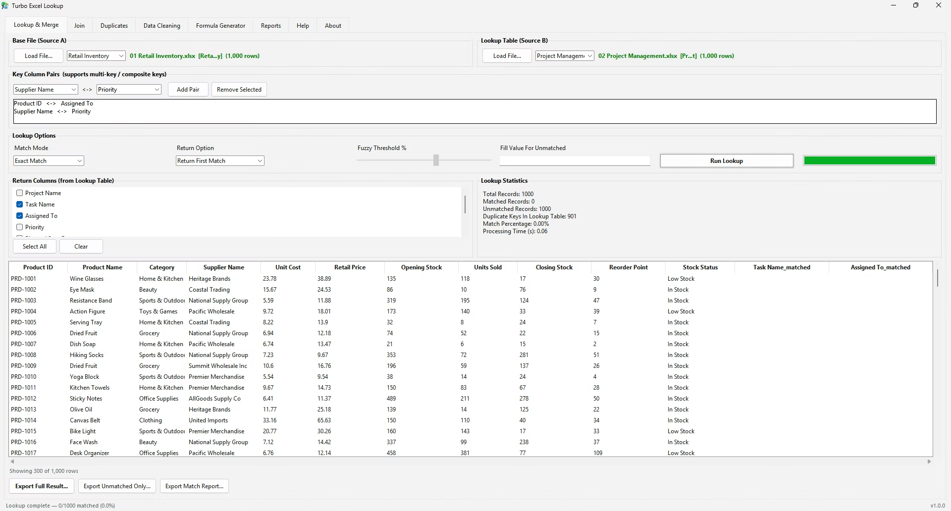
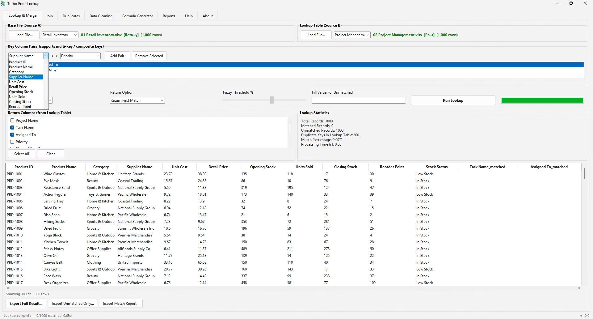
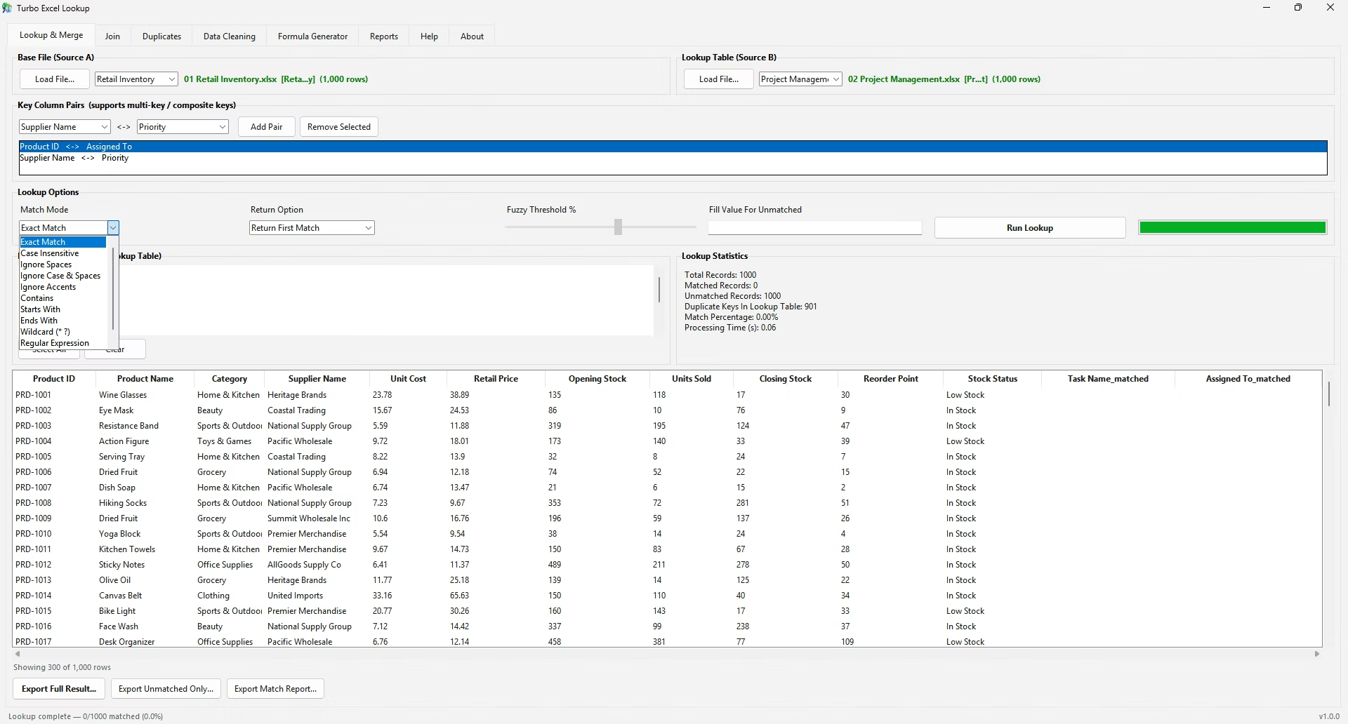
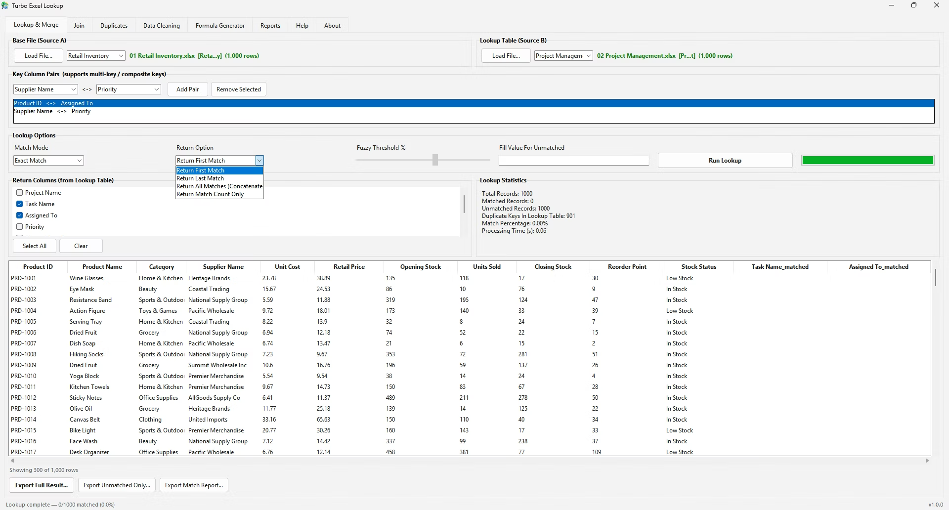
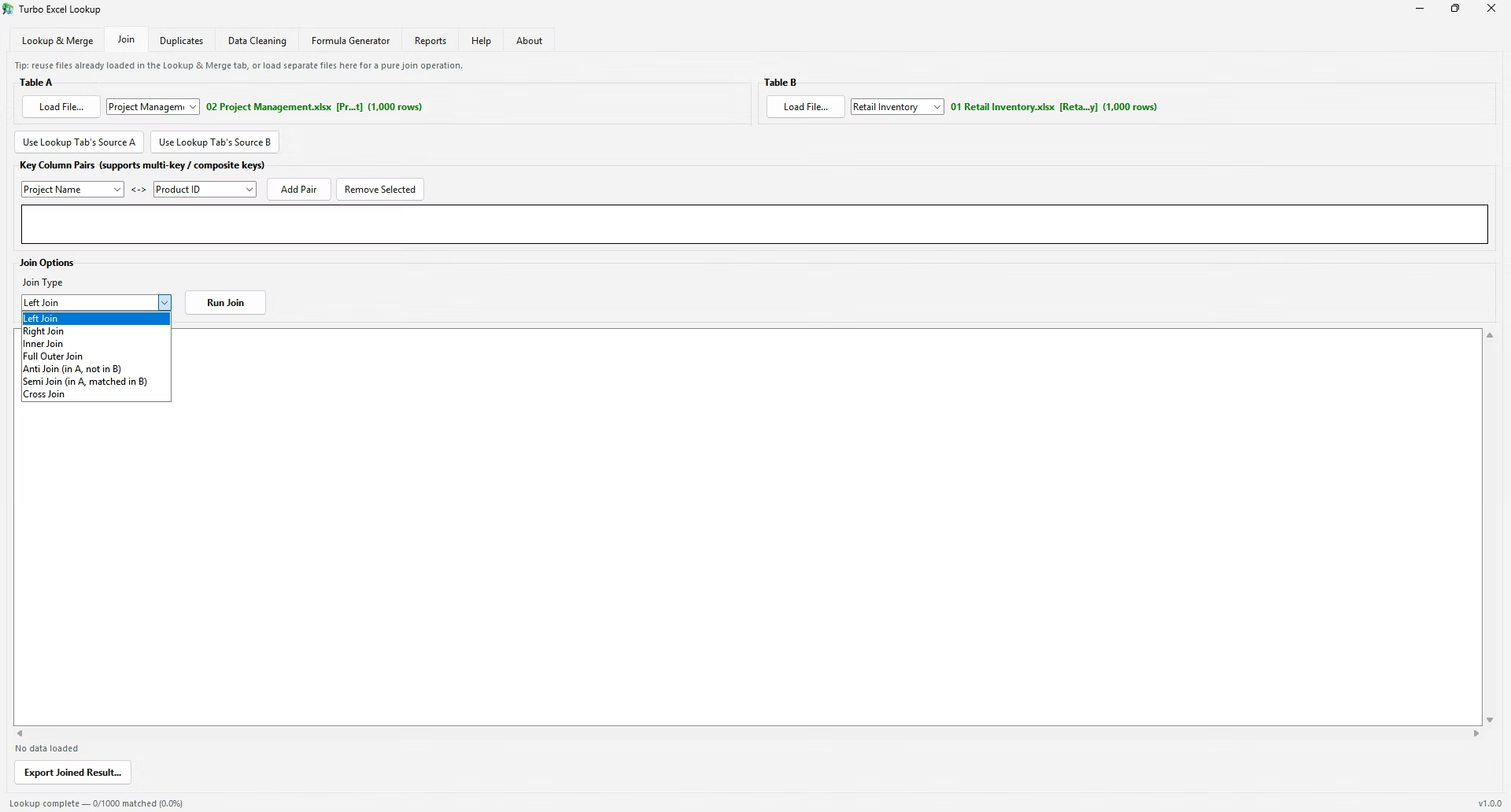
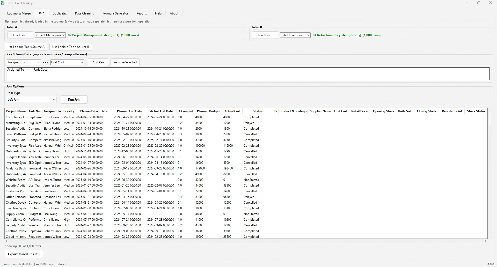
The moment this same lookup needs to run against dozens of SKUs instead of three, or against two separate files, Turbo Excel VLookup handles that scale-up automatically - the underlying matching idea stays exactly this simple, but it runs across the whole dataset at once.
A surprising number of VLOOKUP problems turn out to be a data type mismatch rather than a logic error - a value stored as text in one column and as a number in the other will never match, even if they look identical on screen.
Before assuming the formula itself is wrong, select the lookup value's cell and check the small green triangle or the number alignment; numbers align right by default, and text aligns left, which is a fast way to spot the mismatch.
In a shared workbook, a bare VLOOKUP formula gives the next person no indication of what it's supposed to be matching or why. Adding a cell comment, or a short label in an adjacent column, explaining the source and purpose of the lookup saves significant time when the workbook is revisited months later or handed to a colleague.
This becomes even more important once a workbook has several lookups feeding into each other, since untangling a chain of undocumented formulas is far harder than reading a documented one.
Why use such a small table for the example?
A small table makes it easier to trace exactly what each of the four VLOOKUP arguments is doing without distraction.
What happens if I change col_index_num in the example?
The formula returns a value from a different column in the same matched row, without needing any other argument changed.
Does this simple example work the same way on a larger table?
Yes, the same four-argument pattern applies regardless of table size - only the range in table_array needs to grow.
Why is range_lookup set to FALSE in this example?
Because SKUs are unique identifiers, and an exact match is required to avoid returning the wrong product's data.
What's the next step after understanding this simple example?
Practicing with a real spreadsheet and locking the table_array with F4 before copying the formula down a column.
Is there a way to skip typing the formula for a bigger table?
Yes, Turbo Excel VLookup applies the same simple matching logic automatically across an entire dataset.
Is it a good idea to edit source data while formulas are actively referencing it?
It's safer to keep a stable source sheet separate from a working sheet, since editing referenced data mid-use can produce confusing intermediate results.
Why would a text-formatted number fail to match a real number?
Excel treats text and numeric values as different data types, so "101" stored as text won't match 101 stored as a number even though they display the same.
Does locking a range with F4 change how the formula calculates?
No, it only fixes the range so it doesn't shift when the formula is copied - the calculation itself works the same either way.
What's a fast way to check what a formula is actually returning?
Selecting part of the formula in the formula bar and pressing F9 shows its calculated value directly, without changing the formula.
Ready to stop fighting #N/A errors and match your spreadsheets visually?