This page walks through VLOOKUP one step at a time, using a small invoice table as the running example throughout. Rather than presenting the finished formula and explaining it afterward, each step below builds the formula up one argument at a time so it's clear exactly why each piece is there.
By the last step, the same process can be applied to any two-column matching problem, regardless of what the actual data looks like.

Using this invoice table, the goal is to find the Amount Due for INV-3302:
| Invoice No | Client | Amount Due | Due Date |
|---|---|---|---|
| INV-3301 | Sundar Traders | 24500 | 12-Sep-2026 |
| INV-3302 | Kavya Textiles | 18900 | 20-Sep-2026 |
| INV-3303 | Om Enterprises | 31200 | 28-Sep-2026 |
The value being searched for - the lookup_value - is "INV-3302", and it needs to be found in column A, since that's the leftmost column.
The table_array needs to include the lookup column and every column you might want returned. Here that's A2:D4 - starting at the Invoice No column and extending through Due Date, even though only Amount Due is needed, because col_index_num counts from the start of this range.
Counting from A as 1, B as 2, and so on, Amount Due sits in column C, which is the third column in the selected range. So col_index_num is 3.
Since invoice numbers need to match exactly, the fourth argument is FALSE. Putting it together:
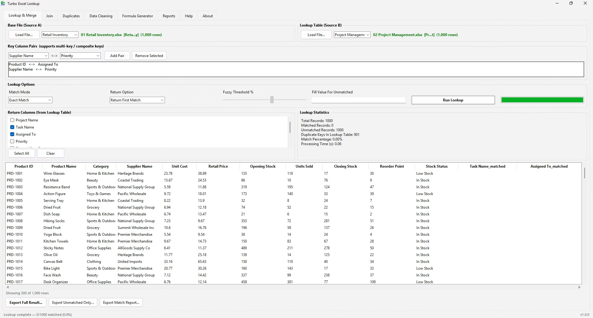
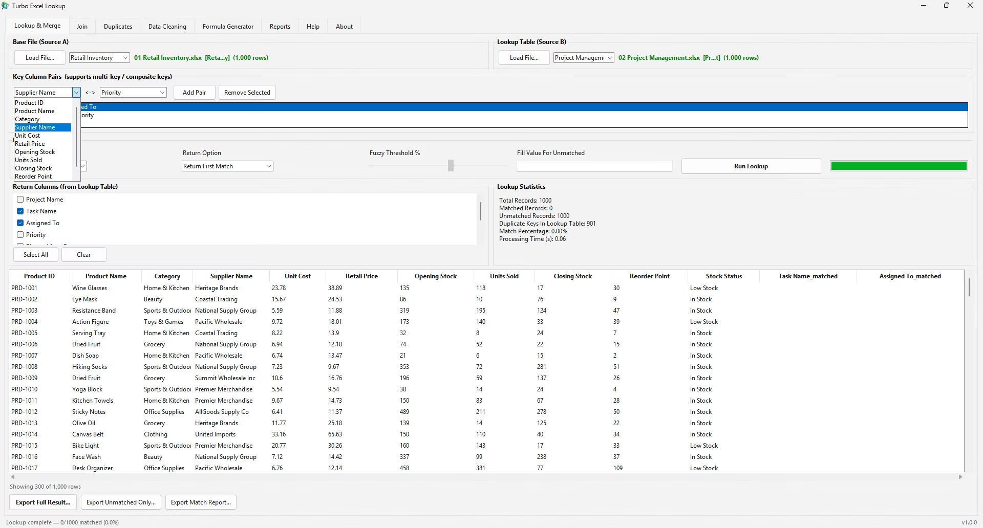
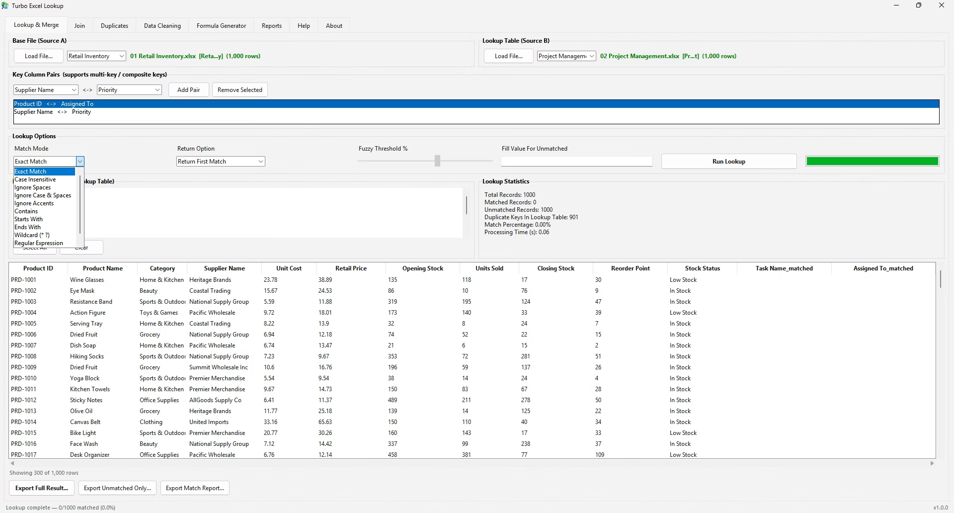
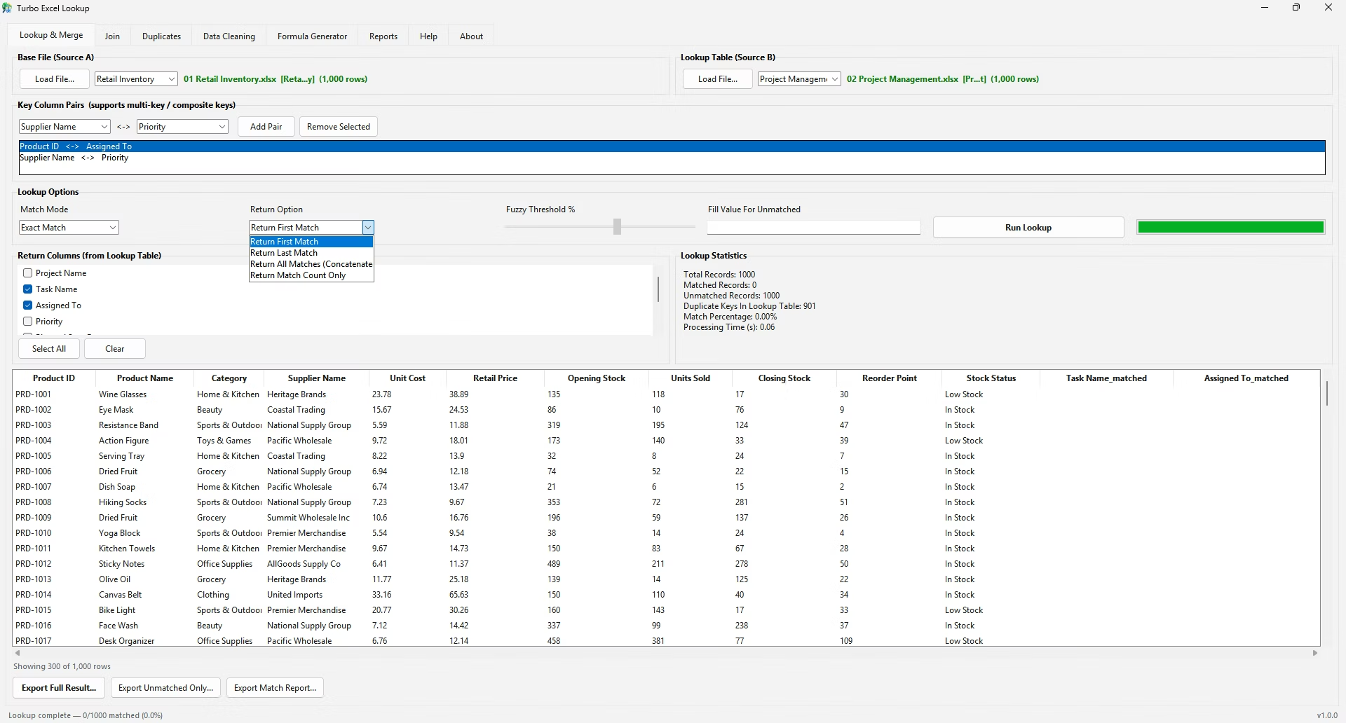
To reuse this formula for a list of invoice numbers, lock the table_array with F4 before copying it down, so every copy still points at A2:D4 rather than shifting. For matching an entire invoice list at once instead of copying formulas, Turbo Excel VLookup runs the same match across the whole file in a single step.
When a VLOOKUP formula that used to work suddenly returns the wrong value with no visible error, the most likely cause is that a column was inserted or deleted inside table_array, shifting col_index_num out of alignment with the intended column.
Selecting the formula and pressing F9 with just that part of the formula highlighted shows the calculated value inline, which is a quick way to confirm whether table_array is still pointing where it should.
A common source of confusing errors is editing the same table that a VLOOKUP formula is pulling from, especially when rows are sorted or filtered mid-edit. Keeping a clearly labeled, rarely edited "source" sheet that formulas pull from, separate from a "working" sheet where day-to-day changes happen, reduces the chance of a lookup silently pulling from a half-edited row.
What is the lookup_value in a VLOOKUP formula?
The value being searched for, which must be found in the leftmost column of the selected data range.
Why does the table_array need to include columns before the one I want?
Because col_index_num is a count of columns starting from the first column of table_array, so it needs the full span included.
How do I count col_index_num correctly?
Count the columns in the selected table_array starting at 1 for the leftmost column, up to the column you want returned.
What happens if I use TRUE instead of FALSE for invoice numbers?
It may return an incorrect nearby match instead of an exact one, which is risky for identifiers like invoice numbers.
Why lock the table_array with F4?
So the range stays fixed when the formula is copied to other cells, instead of shifting down with each row.
Is there a faster way to match every invoice at once?
Yes, Turbo Excel VLookup matches an entire list of invoice numbers in one action rather than copying the formula row by row.
Is it safe to have duplicate values in the lookup column?
A lookup formula will only return the first matching row it finds, so duplicates can silently return the wrong record if not accounted for.
Should I test a new formula on one row before applying it everywhere?
Yes, verifying a single result against the source data first catches setup mistakes before they're copied across an entire column.
Is it a good idea to edit source data while formulas are actively referencing it?
It's safer to keep a stable source sheet separate from a working sheet, since editing referenced data mid-use can produce confusing intermediate results.
Why would a text-formatted number fail to match a real number?
Excel treats text and numeric values as different data types, so "101" stored as text won't match 101 stored as a number even though they display the same.
Ready to stop fighting #N/A errors and match your spreadsheets visually?