An outlier is a value that sits far outside the normal range of the rest of the data in a column - a data-entry error that added an extra zero, a sensor glitch, or a genuinely unusual event that you have decided is not representative for the analysis at hand. Left in place, a single extreme value can pull an average sharply in one direction, stretch a chart's axis so far that the normal data becomes hard to read, and distort statistical measures like standard deviation.
Removing outlier rows is not always the right call - sometimes the outlier is the most important data point in the set - but when the goal is a clean summary of typical behavior, filtering them out first produces a much more representative picture.

One widely used approach is the interquartile range method: calculate the first quartile (QUARTILE.INC with 1) and third quartile (QUARTILE.INC with 3) of a numeric column, find the interquartile range between them, and flag any value more than 1.5 times that range above the third quartile or below the first quartile as an outlier. This method adapts automatically to the natural spread of your specific dataset rather than relying on a fixed cutoff that might not fit every column.
Building this formula correctly takes a bit of care, since it needs to reference the right column consistently down every row while the quartile boundaries themselves stay fixed.
A common mistake is applying a single outlier threshold across an entire sheet when different columns naturally have very different scales and distributions - a value that is extreme in one column might be perfectly normal in another. It is also worth resisting the temptation to remove every flagged row automatically without a quick manual review first, since a statistical outlier is sometimes the most important and correct data point in the entire dataset.
- In an empty cell, calculate Q1 with =QUARTILE.INC(B:B,1) and Q3 with =QUARTILE.INC(B:B,3).
- Calculate the interquartile range as Q3 minus Q1 in another cell.
- Add a helper column with a formula that flags TRUE when a row's value falls outside Q1 minus 1.5×IQR to Q3 plus 1.5×IQR.
- Filter the helper column to show only TRUE rows and review them before deleting.
- Delete the confirmed outlier rows, then remove the helper column and calculations.
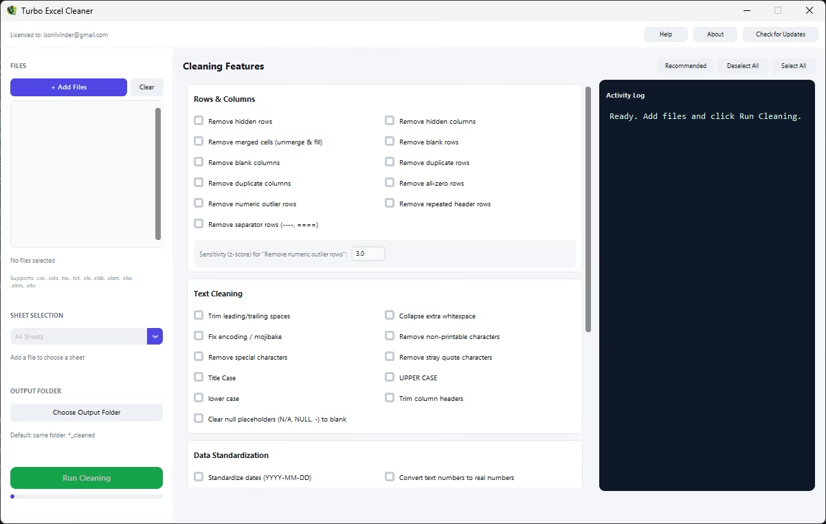
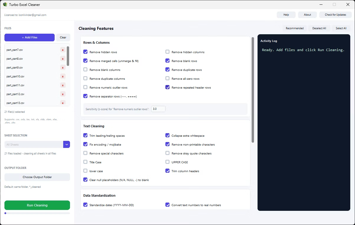
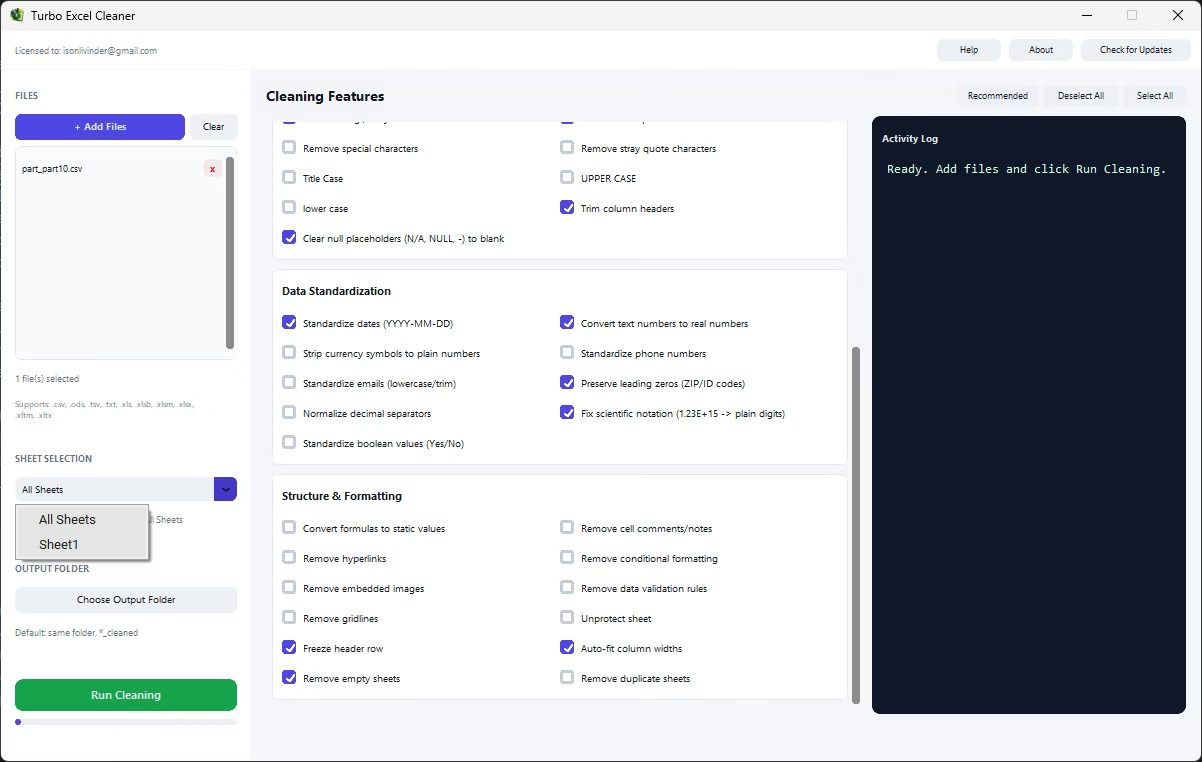
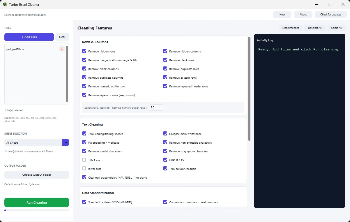
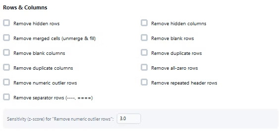
Building and re-checking quartile formulas by hand for every new file is time-consuming, especially across a batch of similar reports that each need the same statistical check applied. Turbo Excel Cleaner's Remove Numeric Outlier Rows feature applies a statistical outlier check to your numeric columns automatically, removing rows with extreme values without requiring you to write or debug a formula.
As with the rest of the app's Rows & Columns category, this feature can be combined with all-zero row removal and blank row removal in the same run, giving you a dataset trimmed of both dead rows and statistically extreme rows in one pass.
- Automatic statistical outlier detection for numeric columns
- No manual quartile formulas to build or maintain
- Combine with other Rows & Columns features in one run
- Applied consistently across every sheet in a batch of files
- Works on Excel, OpenDocument, CSV, TSV, and TXT files
Will this remove legitimate but unusual data?
Outlier detection is a statistical judgment, not a certainty - it is a good idea to review a sample of the flagged rows against your knowledge of the data before relying on the cleaned file for critical analysis.
Does outlier detection work on text columns?
No, outlier detection applies specifically to numeric columns, since the concept of a statistical outlier requires values that can be compared and ranked.
Can I apply this to only some columns in a sheet?
The feature evaluates the numeric columns present in each row; reviewing the cleaned output lets you confirm the behavior matches what your specific dataset needs.
Ready to clean your spreadsheets in bulk, offline, with full privacy?