VLOOKUP looks intimidating the first time you see it written out, but the idea behind it is simple: give Excel something to search for, tell it where to search, and tell it which column to bring back. Once that idea clicks, the formula itself is mostly just filling in four blanks in the right order.
This page walks through an easy version of VLOOKUP using a small employee table, then shows how Turbo Excel VLookup lets you skip the formula altogether if the syntax still feels awkward after a few tries.
Every VLOOKUP formula asks for the same four pieces of information, in the same order every time: the value you're searching for, the range that contains your data, the position (counted in columns) of the value you want returned, and whether you need an exact or approximate match.
Once you can identify those four pieces in plain English before touching the formula bar, typing the actual formula becomes a lot less stressful.
Say you have this small employee table and want to find the Department for employee E102:
| Employee ID | Name | Department | Salary |
|---|---|---|---|
| E101 | Asha Rao | Marketing | 54000 |
| E102 | Vikram Shah | Finance | 61000 |
| E103 | Priya Nair | Sales | 48000 |
The formula below searches column A for "E102", then counts three columns to the right to return the Department value.
The single most common mistake is forgetting the FALSE at the end, which allows Excel to return an approximate match instead of an exact one - often resulting in the wrong row entirely.
The second most common mistake is selecting a table_array that starts to the right of the lookup column. VLOOKUP can only search the first column of whatever range you give it, so the ID column always needs to be the leftmost column in your selection.
If you plan to copy the formula down a column, press F4 after selecting the table_array to add dollar signs and lock the range in place. Without this step, the range shifts down with each copied row and the formula eventually points at empty cells.
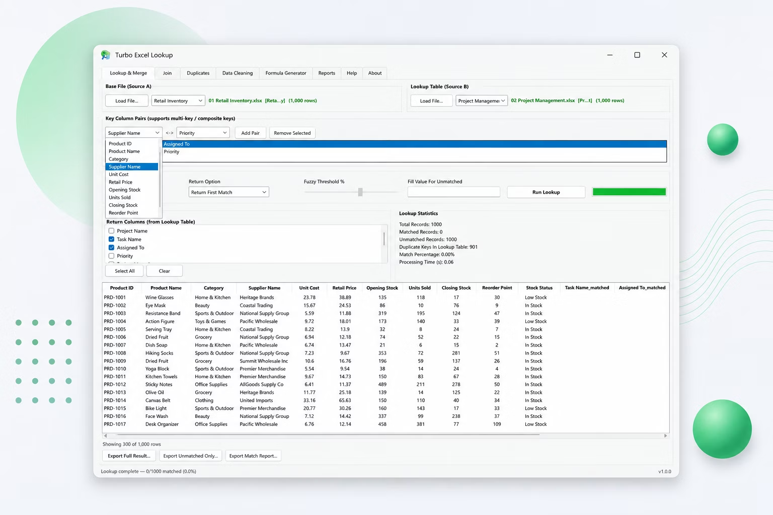
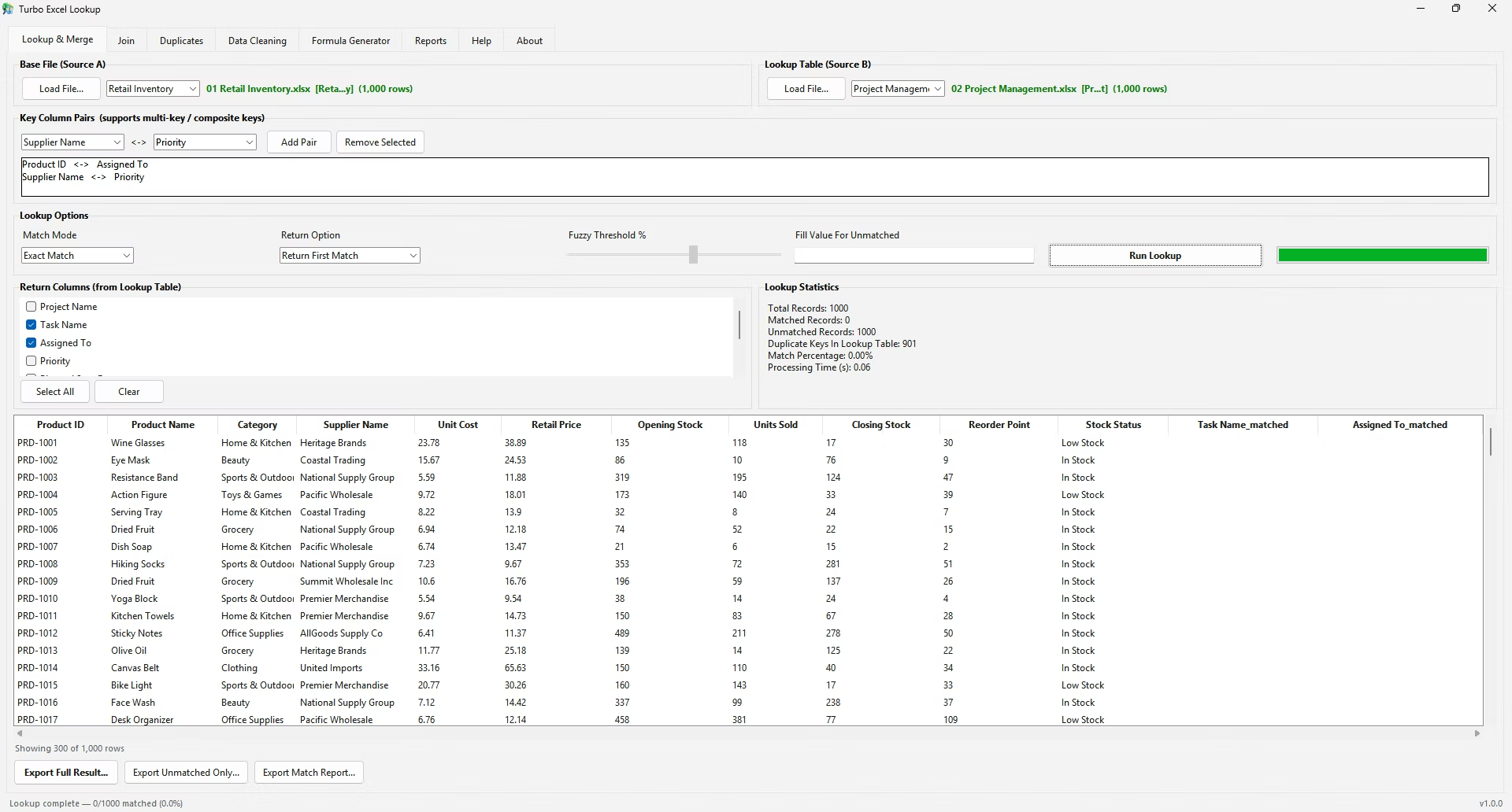
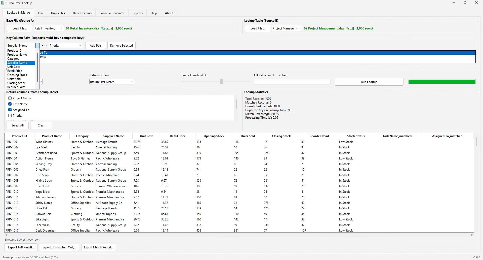
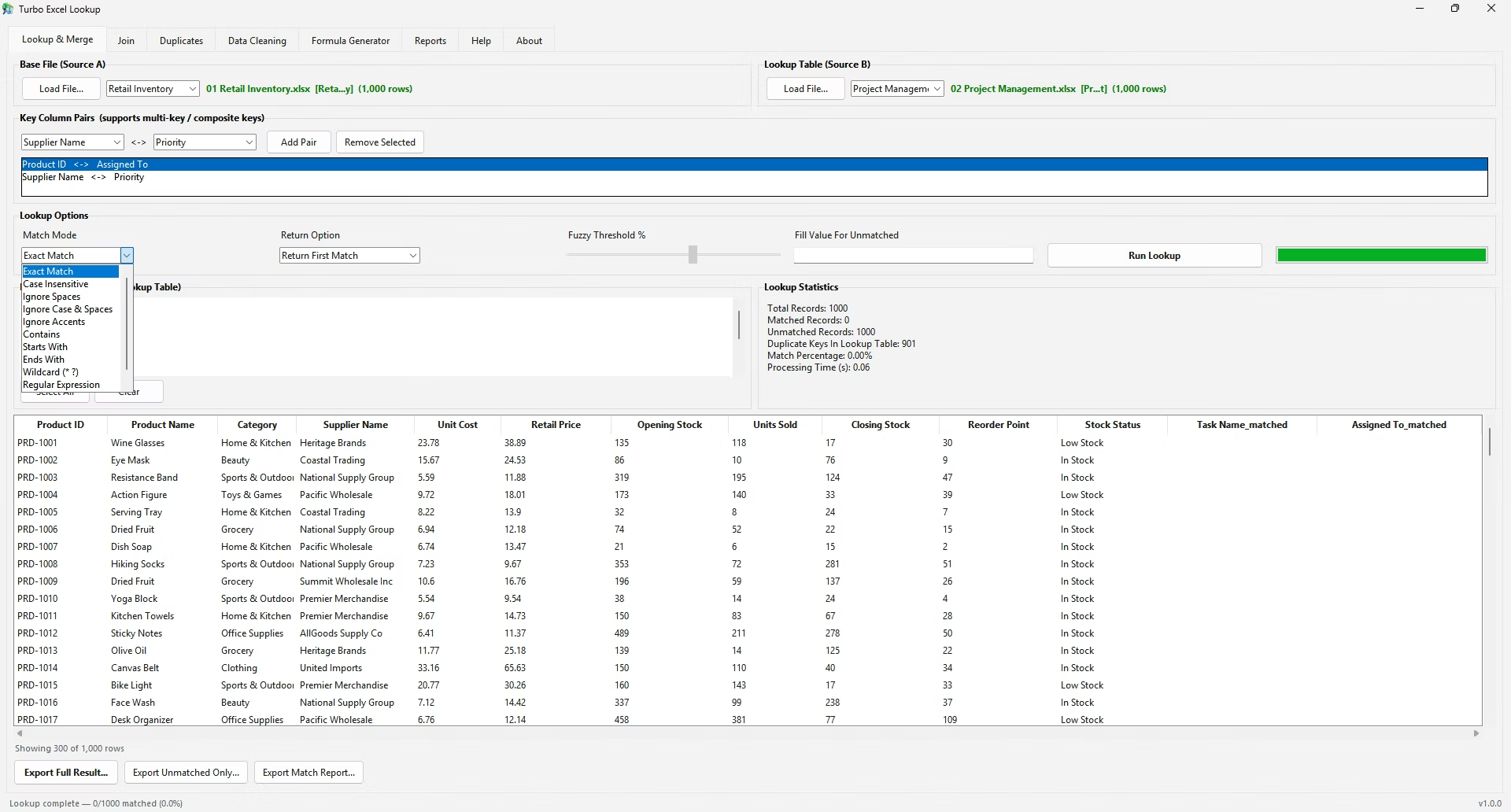
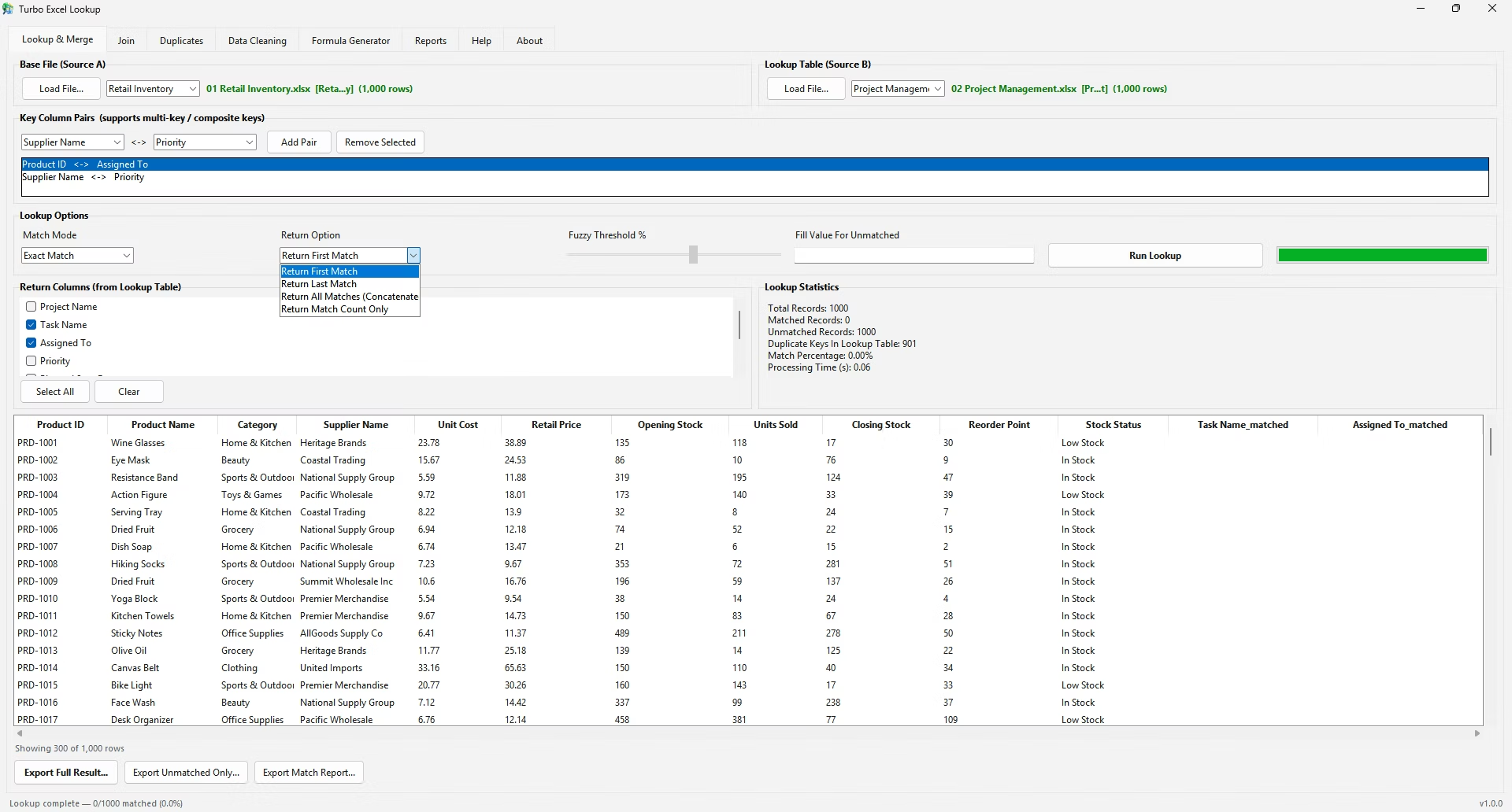
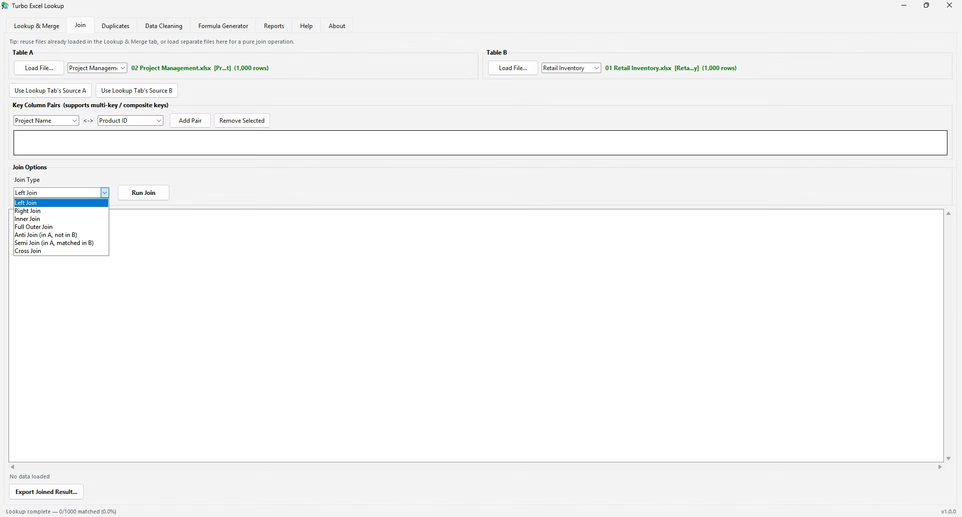
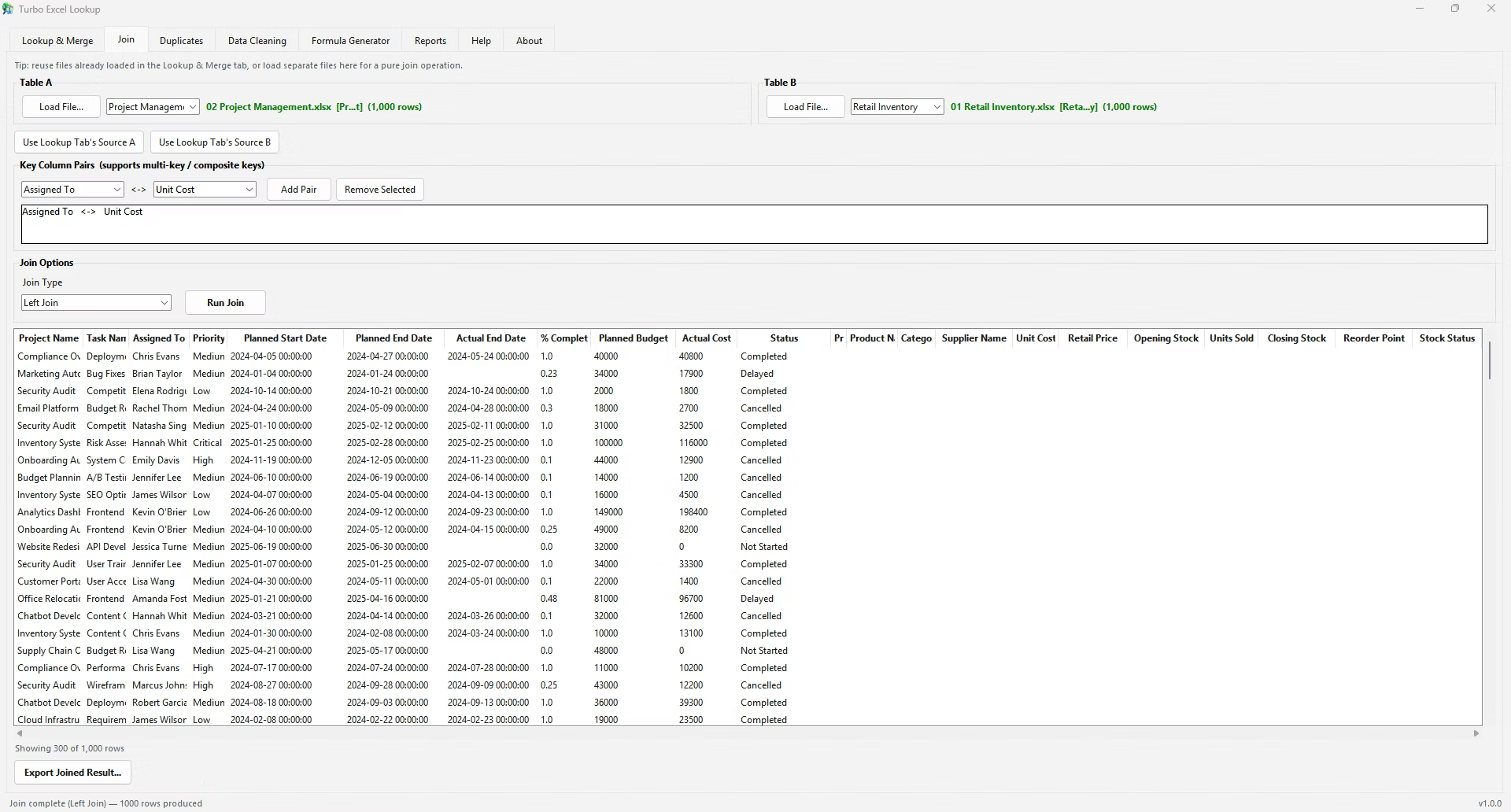
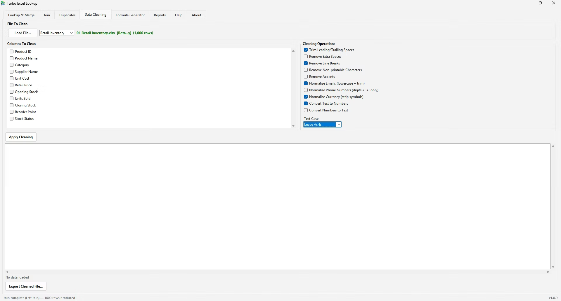
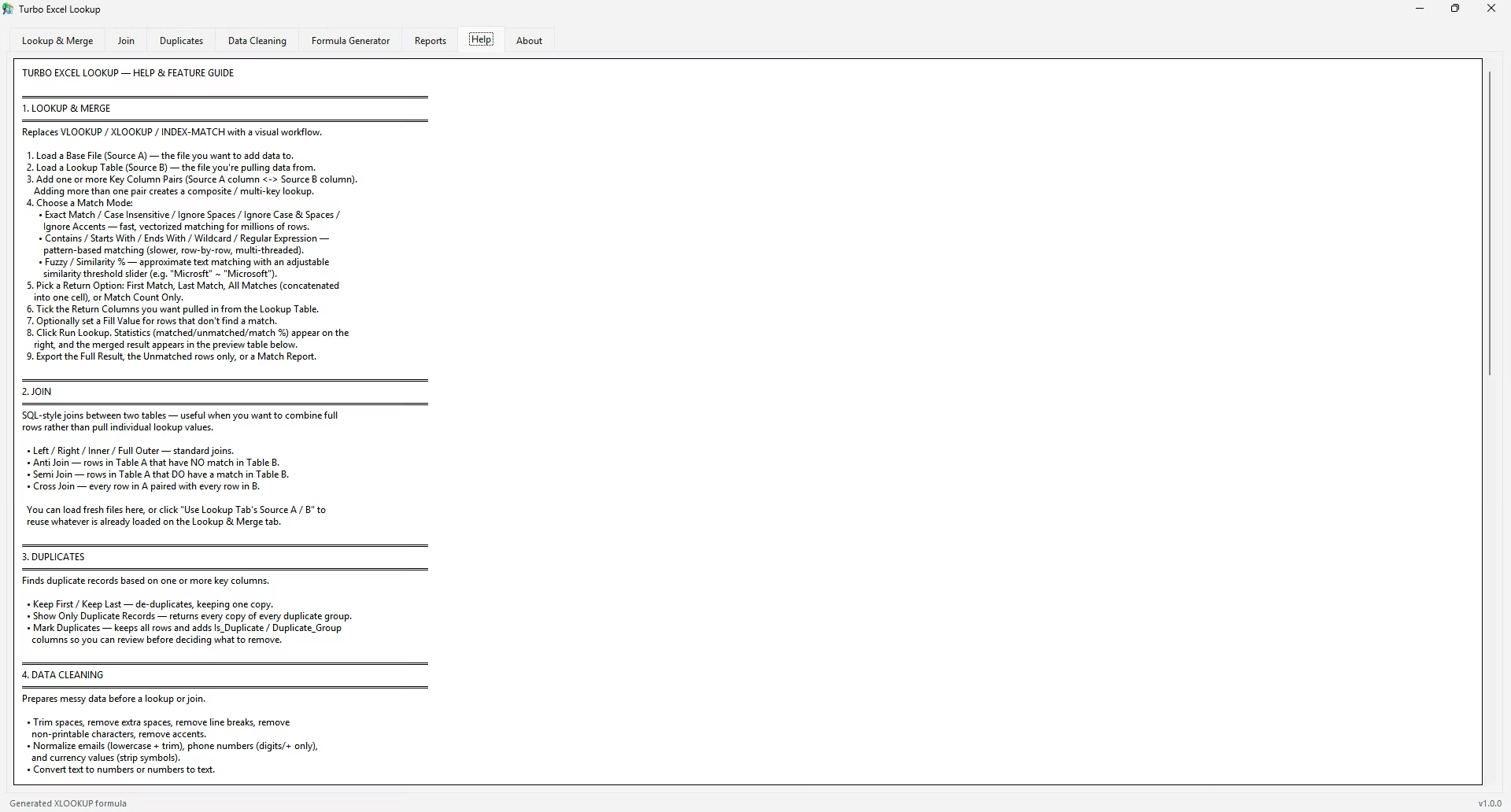
Turbo Excel VLookup was built for exactly this situation. Instead of typing a formula, you load your base file and lookup table, pick the matching ID columns from two dropdown menus, tick the columns you want returned, and click Run Lookup. It matches the entire dataset in one pass, so there's no formula to copy down and no risk of the range slipping.
A worksheet with thousands of VLOOKUP formulas recalculating against a large table_array can slow Excel down noticeably, especially if the range isn't locked and Excel has to re-evaluate a shifting reference on every keystroke.
Converting the source range into an Excel Table (Insert > Table) before referencing it in VLOOKUP tends to help, since Table references automatically resize with the data and stay consistent without needing manual $ locking.
Before applying a new VLOOKUP formula to an entire column, it's worth testing it on a single row and manually verifying the result against the source data, since a mistake caught in one cell takes seconds to fix, while the same mistake copied down five hundred rows takes much longer to untangle.
This is especially worth doing whenever the source table_array has changed shape recently, since a resized or reordered table is the single most common reason a previously reliable formula starts returning unexpected results.
What are the four arguments in VLOOKUP?
The value to search for, the range containing the data, the column number to return, and TRUE or FALSE for approximate or exact match.
Why does my VLOOKUP return the wrong value?
This usually happens when FALSE is left out, allowing an approximate match, or when the lookup column isn't the leftmost column in the selected range.
Do I need to lock the table_array with $ signs?
Only if you plan to copy the formula to other cells - locking it with F4 keeps the range from shifting as you copy down.
Can VLOOKUP search to the left of the ID column?
No, standard VLOOKUP only searches the leftmost column of the selected range; INDEX MATCH or XLOOKUP is needed to search leftward.
What does #N/A mean in a VLOOKUP result?
It means Excel searched the lookup column and found no exact match for the value you gave it, often due to typos or extra spaces.
Is there a way to avoid typing the formula at all?
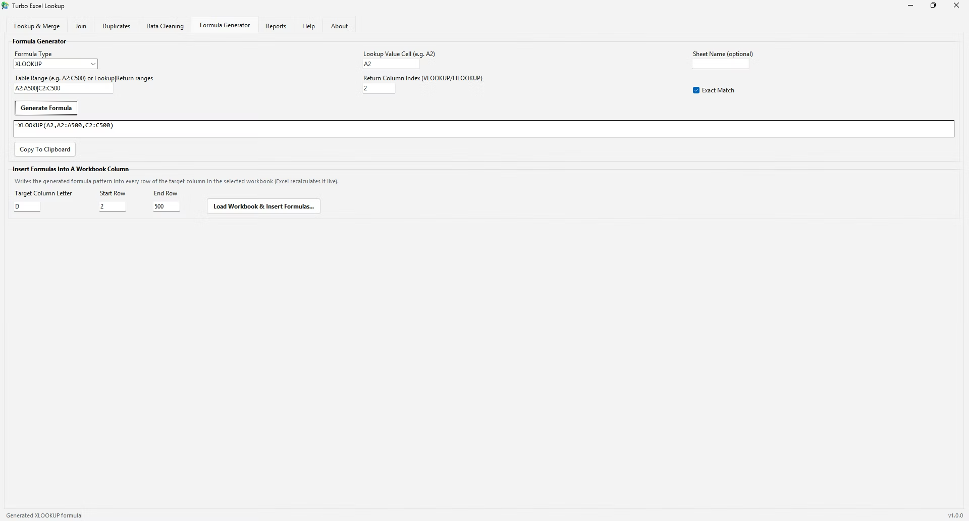
Yes, Turbo Excel VLookup performs the same matching through a point-and-click interface without requiring any formula to be written.
Why would a text-formatted number fail to match a real number?
Excel treats text and numeric values as different data types, so "101" stored as text won't match 101 stored as a number even though they display the same.
Does locking a range with F4 change how the formula calculates?
No, it only fixes the range so it doesn't shift when the formula is copied - the calculation itself works the same either way.
What's a fast way to check what a formula is actually returning?
Selecting part of the formula in the formula bar and pressing F9 shows its calculated value directly, without changing the formula.
Can trailing spaces in a cell cause a lookup to fail?
Yes, an extra space at the end of a value is invisible but prevents an exact match; TRIM() around the lookup value often fixes this.
Ready to stop fighting #N/A errors and match your spreadsheets visually?